Estimating covariate diffusion with sdmTMB

If the code in this vignette has not been evaluated, a rendered version is available on the documentation site under ‘Articles’.

library(ggplot2)
library(sdmTMB)
theme_set(theme_light())

This vignette demonstrates covariate-diffusion models using simulated data. These models could alternatively be described as “distributed lag” models.

When might you want to fit these models? Sometimes, the spatial or temporal scale at which covariates influence the response is unclear.

For example, fish move. Therefore, if we measure temperature at the location where a fish was sampled, it may be unclear whether the model should use the temperature at the sampling site or a smoothed version of the temperature surface that accounts for fish movement and integration over a broader spatial range.

One option is to fit models using covariates with different levels of smoothing and compare them. Alternatively, we can estimate the appropriate degree of smoothing simultaneously with the parameters of the main model. This is what the covariate-diffusion functionality does.

Users are encouraged to read and cite Lindmark et al. (2025) for spatial models and Thorson et al. (2026) for extensions to temporal and spatiotemporal settings, including the introduction of the MSD and RMSD terms.

We begin with a simple spatial-diffusion example and then fit an example that combines space() and time() terms.

Simple spatial diffusion example

We will start by simulating data with a fine-scale predictor (x1) and a spatially diffused effect:

set.seed(1)
n_sites <- 220
site <- data.frame(X = runif(n_sites), Y = runif(n_sites))
dat <- transform(
  site,
  x1 = as.numeric(scale(
    sin(6 * pi * X) + cos(6 * pi * Y) + rnorm(n_sites, sd = 1)
  ))
)
mesh <- make_mesh(dat, c("X", "Y"), cutoff = 0.05)

sim_space <- simulate_new(
  formula = ~ 1,
  data = dat,
  mesh = mesh,
  family = gaussian(),
  spatial = "off",
  spatiotemporal = "off",
  range = 0.2,
  sigma_O = 0,
  phi = 0.1,
  B = c(0, 0.8),
  covariate_diffusion = ~ space(x1),
  diffusion_kappaS = 1.5,
  seed = 1
)

dat$observed <- sim_space$observed
dat$x1_truth <- sim_space$diffusion_truth_space_x1
head(dat)
#>           X         Y          x1    observed     x1_truth
#> 1 0.2655087 0.2624741 -1.80218040 -0.05509372  0.009439577
#> 2 0.3721239 0.1654539 -0.21021214  0.01510442 -0.004074891
#> 3 0.5728534 0.3221681 -0.43693836 -0.07591271  0.009562691
#> 4 0.9082078 0.5101252 -1.69168657  0.13020238 -0.036657119
#> 5 0.2016819 0.9239685 -1.18474680  0.06744091  0.043112665
#> 6 0.8983897 0.5109597 -0.05084862 -0.10927063 -0.034029739

Fit the matching covariate-diffusion model:

fit <- sdmTMB(
  observed ~ 1,
  mesh = mesh,
  covariate_diffusion = ~ space(x1), #<
  spatial = "off",
  data = dat
)

fit
#> Model fit by ML ['sdmTMB']
#> Formula: observed ~ 1
#> Mesh: mesh (isotropic covariance)
#> Data: dat
#> Covariate diffusion: space(x1)
#> Family: gaussian(link = 'identity')
#>  
#> Conditional model:
#>                   coef.est coef.se
#> (Intercept)           0.01    0.01
#> cov_diff_space_x1     0.23    0.15
#> 
#> Dispersion parameter: 0.09
#> Covariate diffusion RMSD: RMSD[x1]=0.46
#> ML criterion at convergence: -207.521
#> 
#> See ?tidy.sdmTMB to extract these values as a data frame.
tidy(fit)
#> # A tibble: 2 × 5
#>   term              estimate std.error  conf.low conf.high
#>   <chr>                <dbl>     <dbl>     <dbl>     <dbl>
#> 1 (Intercept)         0.0138   0.00675  0.000551    0.0270
#> 2 cov_diff_space_x1   0.226    0.149   -0.0658      0.517
tidy(fit, effects = "ran_pars")
#> # A tibble: 4 × 5
#>   term                estimate std.error conf.low conf.high
#>   <chr>                  <dbl>     <dbl>    <dbl>     <dbl>
#> 1 phi                   0.0942   0.00449  0.0858      0.103
#> 2 kappaS_cov_diff[x1]   4.30     2.23    -0.0661      8.67 
#> 3 MSD[x1]               0.216    0.224   -0.223       0.655
#> 4 RMSD[x1]              0.465    0.241   -0.00714     0.937

Here kappaS_cov_diff[x1] is the estimated spatial diffusion scale parameter for x1 (larger values imply less smoothing).

The output also reports MSD[x1] and RMSD[x1], the implied mean squared displacement (4 / kappaS_cov_diff[x1]^2) and root mean squared displacement (2 / kappaS_cov_diff[x1]). RMSD[x1] is a typical diffusion distance (a blur radius) in coordinate units. Users applying this spatial diffusion method should cite Lindmark et al. (2025). Users using these MSD and RMSD metrics should consult and cite Thorson et al. (2026).

Compare true and estimated diffused covariates:

pred <- predict(fit)
pred$X <- dat$X
pred$Y <- dat$Y

cor(pred$diffusion_cov_space_x1, pred$x1_truth)
#> [1] 0.9215819

g1 <- ggplot(pred, aes(X, Y, colour = x1)) +
  geom_point(size = 0.7) +
  scale_colour_gradient2() +
  coord_equal() +
  ggtitle("Fine-scale observed predictor (x1)")

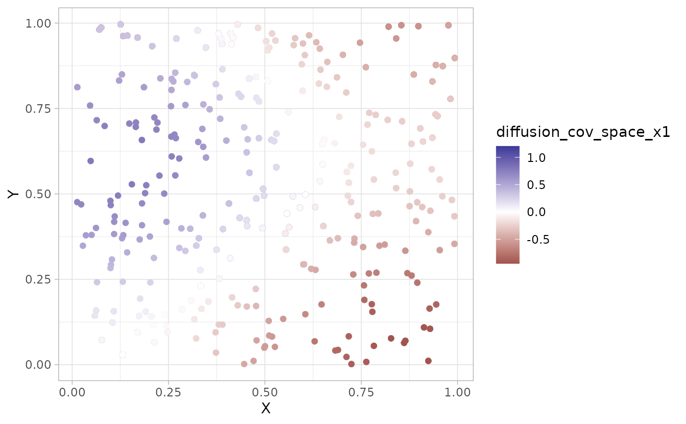
g2 <- ggplot(pred, aes(X, Y, colour = x1_truth)) +
  geom_point(size = 0.7) +
  scale_colour_gradient2() +
  coord_equal() +
  ggtitle("True diffused covariate (from simulation)")

g3 <- ggplot(pred, aes(X, Y, colour = diffusion_cov_space_x1)) +
  geom_point(size = 0.7) +
  scale_colour_gradient2() +
  coord_equal() +
  ggtitle("Estimated diffused covariate")

print(g1)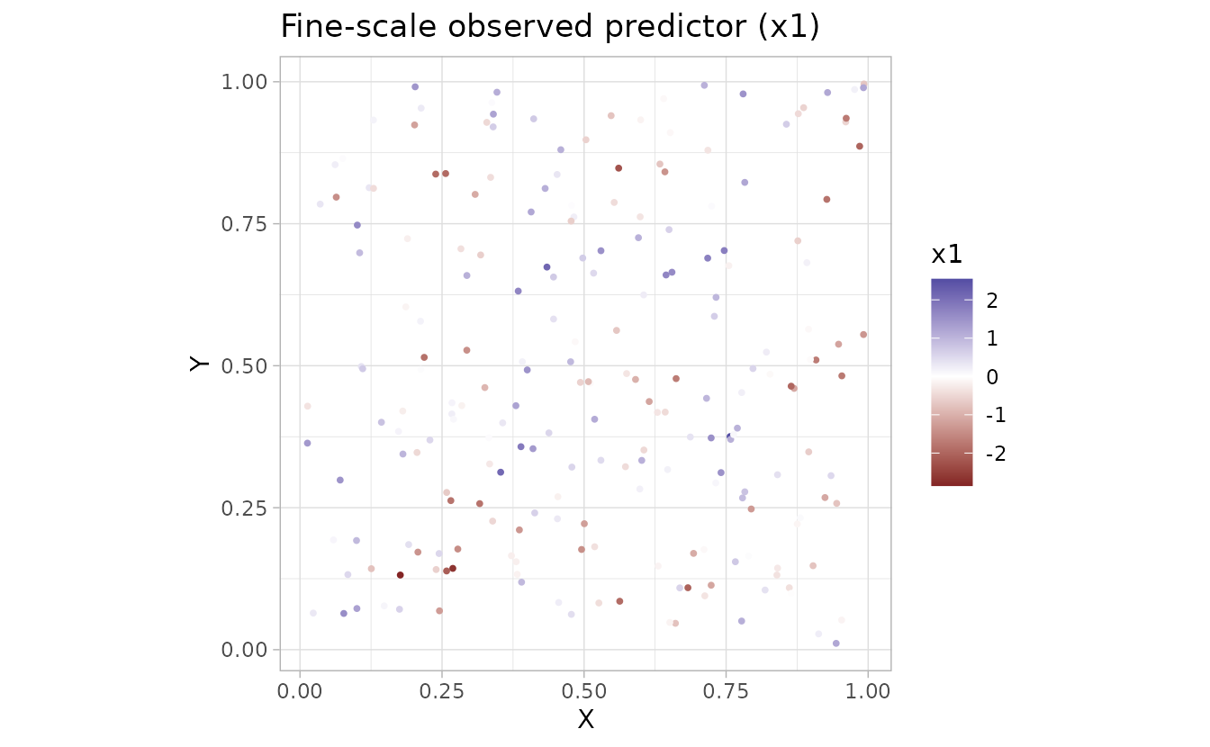

print(g2)

print(g3)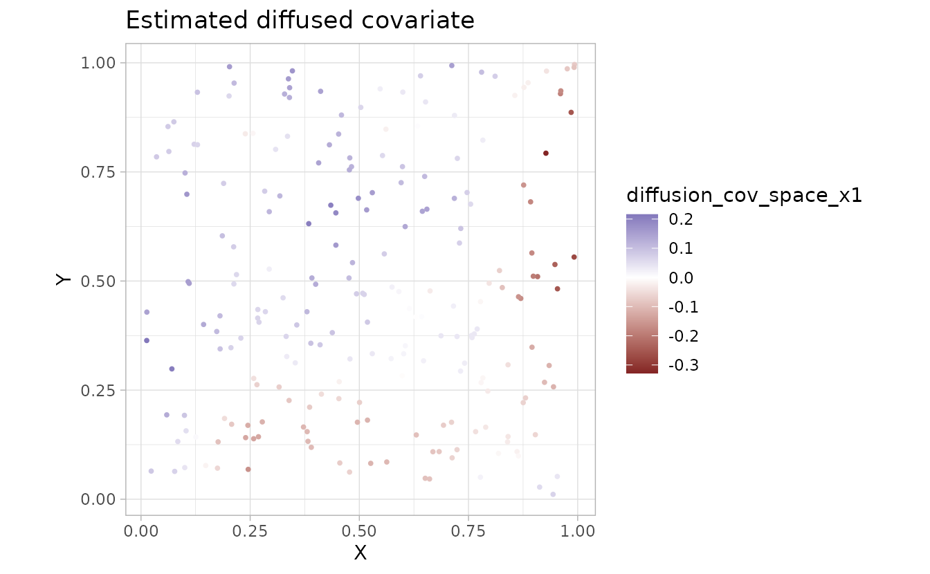

We can visualize the diffusion operator and the original and smoothed covariate on the mesh:

plot_diffusion_kernel(fit, component = "space")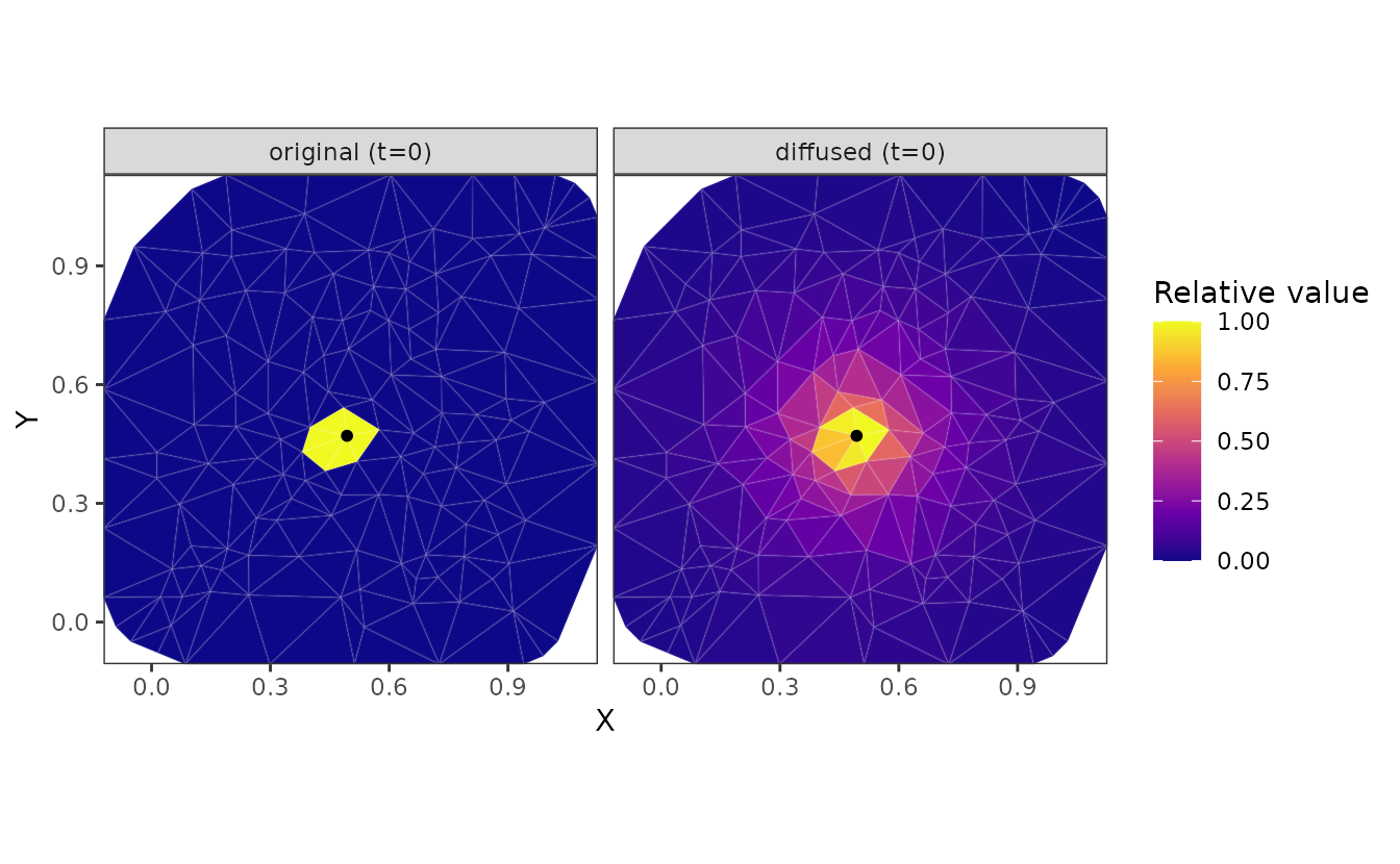

plot_diffused_covariate(fit, component = "space")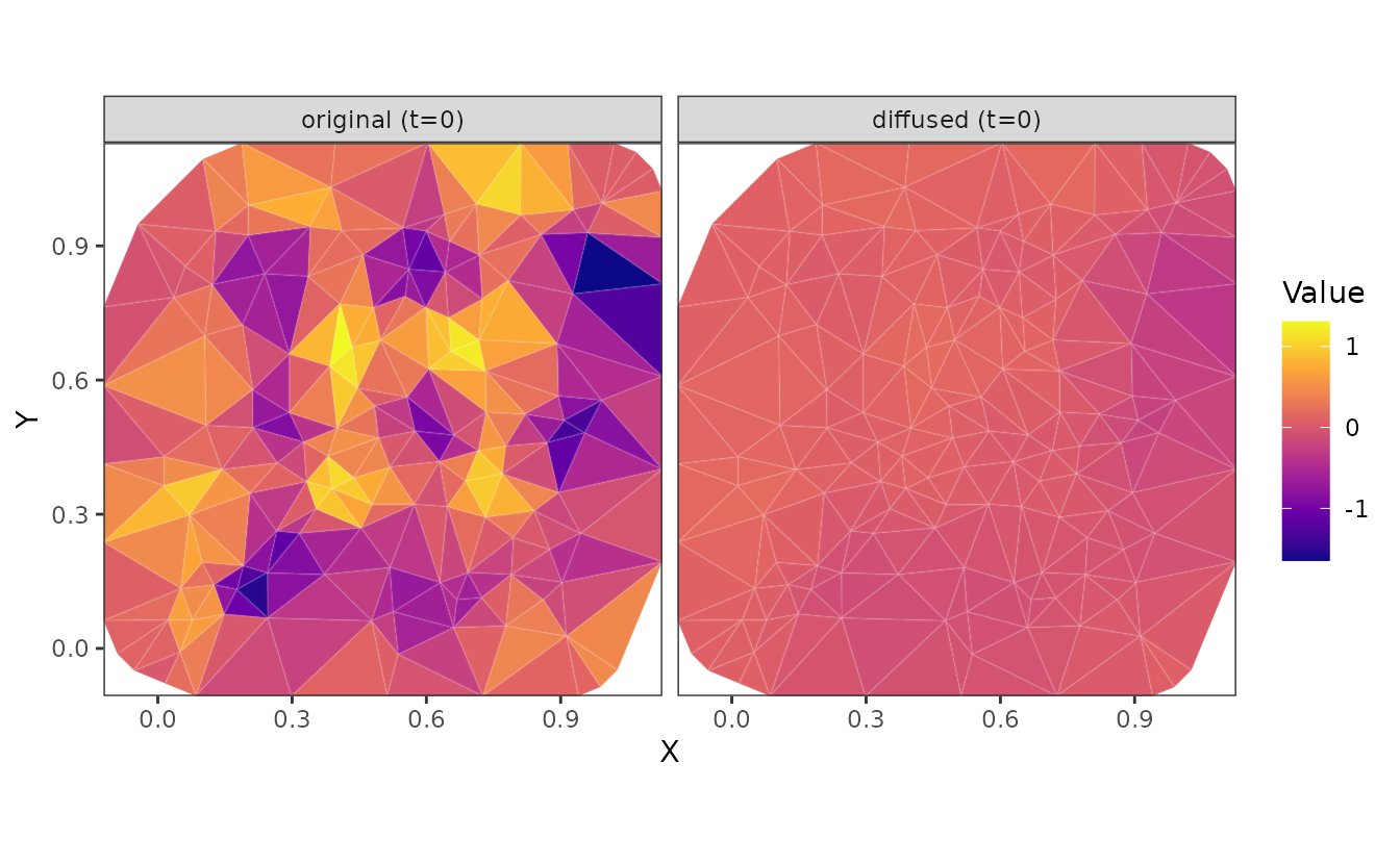

Space-time example with additive terms

Next we will simulate and fit a model containing spatial and temporal components: ~ space(x1) + time(x1).

set.seed(1)
n_t <- 16
n_sites <- 300
site_st <- data.frame(X = runif(n_sites), Y = runif(n_sites))
dat_st <- data.frame(
  X = rep(site_st$X, times = n_t),
  Y = rep(site_st$Y, times = n_t),
  year = rep(seq_len(n_t), each = n_sites)
)
dat_st$x1 <- as.numeric(scale(
  sin(2 * pi * (dat_st$X + dat_st$year / 8)) +
    cos(2 * pi * (dat_st$Y - dat_st$year / 10)) +
    0.6 * sin(4 * pi * dat_st$X) * cos(dat_st$year / 3) +
    rnorm(nrow(dat_st), sd = 0.15)
))
mesh_st <- make_mesh(dat_st, c("X", "Y"), cutoff = 0.07)

sim_st <- simulate_new(
  formula = ~ 1,
  data = dat_st,
  mesh = mesh_st,
  time = "year",
  family = gaussian(),
  spatial = "on",
  spatiotemporal = "off",
  range = 0.3,
  sigma_O = 0.2,
  phi = 0.1,
  B = c(0, 0.7, 0.6),
  covariate_diffusion = ~ space(x1) + time(x1),
  diffusion_kappaS = 4.4,
  diffusion_rhoT = 0.3,
  seed = 123
)

dat_st$observed <- sim_st$observed

fit_st <- sdmTMB(
  observed ~ 1,
  mesh = mesh_st,
  time = "year",
  covariate_diffusion = ~ space(x1) + time(x1), #<
  spatial = "on",
  spatiotemporal = "off",
  data = dat_st
)

sanity(fit_st)
#> ✔ Non-linear minimizer suggests successful convergence
#> ✔ Hessian matrix is positive definite
#> ✔ No extreme or very small eigenvalues detected
#> ✔ No gradients with respect to fixed effects are >= 0.001
#> ✔ No fixed-effect standard errors are NA
#> ✔ No standard errors look unreasonably large
#> ✔ No sigma parameters are < 0.01
#> ✔ No sigma parameters are > 100
#> ✔ Range parameter doesn't look unreasonably large
fit_st
#> Spatial model fit by ML ['sdmTMB']
#> Formula: observed ~ 1
#> Mesh: mesh_st (isotropic covariance)
#> Time column: character
#> Data: dat_st
#> Covariate diffusion: space(x1) + time(x1)
#> Family: gaussian(link = 'identity')
#>  
#> Conditional model:
#>                   coef.est coef.se
#> (Intercept)           0.01    0.05
#> cov_diff_space_x1     0.69    0.01
#> cov_diff_time_x1      0.61    0.01
#> 
#> Dispersion parameter: 0.10
#> Covariate diffusion temporal persistence: rhoT[x1]=0.30
#> Matérn range: 0.28
#> Spatial SD: 0.17
#> Covariate diffusion RMSD: RMSD[x1]=0.38
#> ML criterion at convergence: -4055.260
#> 
#> See ?tidy.sdmTMB to extract these values as a data frame.

tidy(fit_st, effects = "ran_pars")
#> # A tibble: 8 × 5
#>   term                estimate std.error conf.low conf.high
#>   <chr>                  <dbl>     <dbl>    <dbl>     <dbl>
#> 1 range                 0.279    0.0504    0.196      0.398
#> 2 phi                   0.0997   0.00103   0.0977     0.102
#> 3 sigma_O               0.173    0.0175    0.142      0.211
#> 4 kappaS_cov_diff[x1]   4.35     0.103     4.15       4.55 
#> 5 kappaT_cov_diff[x1]   0.431    0.0100    0.411      0.450
#> 6 rhoT[x1]              0.301    0.00490   0.291      0.311
#> 7 MSD[x1]               0.148    0.00771   0.133      0.163
#> 8 RMSD[x1]              0.384    0.0100    0.365      0.404

In the random-effect parameters, kappaS_cov_diff[x1] controls spatial smoothing and kappaT_cov_diff[x1] controls temporal diffusion. Users applying the time diffusion extension should read and cite Thorson et al. (2026).

Plot diffusion kernels

We can separately visualize the spatial diffusion, time diffusion, or their combined effects as either the diffusion kernel or the smoothed covariate field represented on the mesh:

plot_diffusion_kernel(fit_st, component = "space")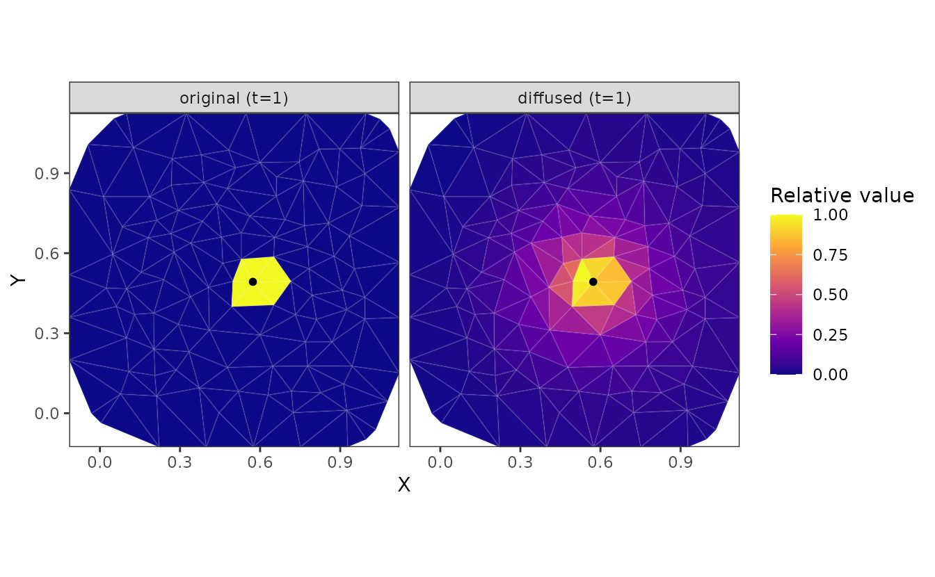

plot_diffusion_kernel(fit_st, component = "time", common_scale = TRUE)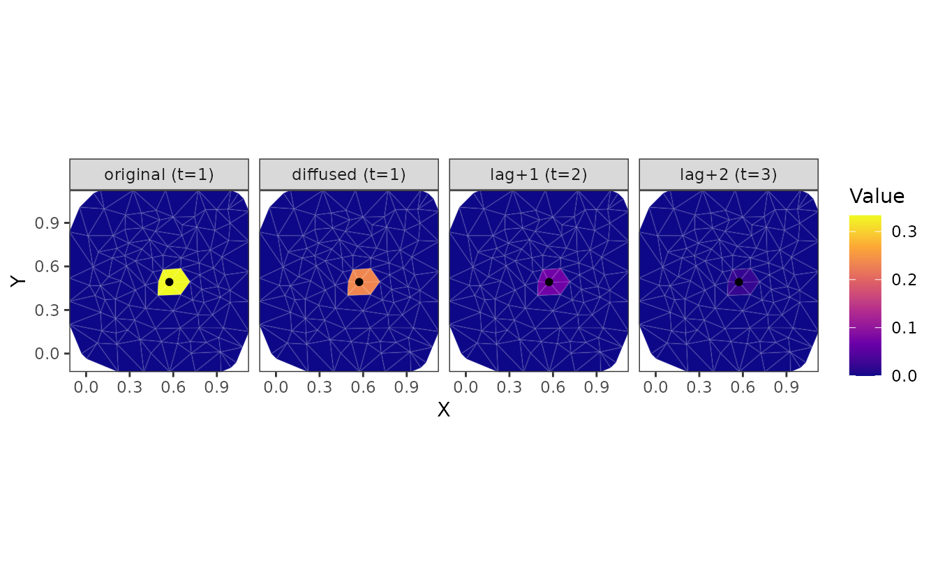

plot_diffusion_kernel(fit_st, component = "combined")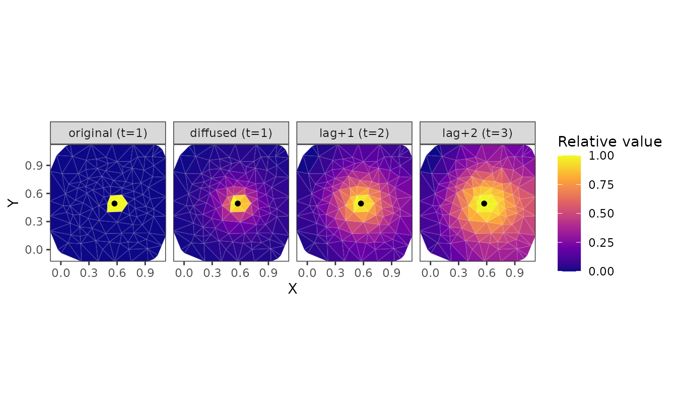

plot_diffusion_kernel(fit_st, component = "combined", common_scale = TRUE)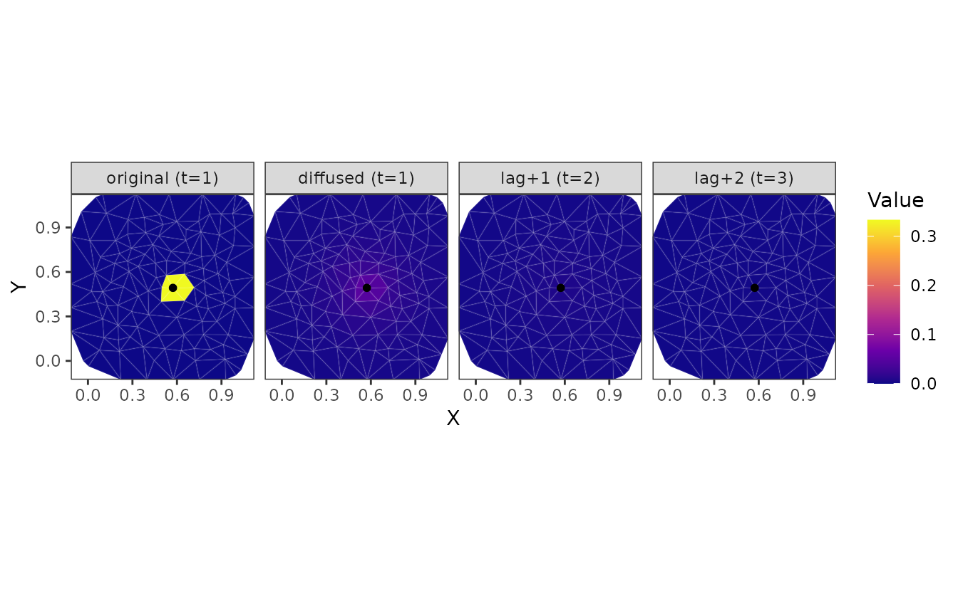

plot_diffused_covariate(fit_st, component = "space")

plot_diffused_covariate(fit_st, component = "time")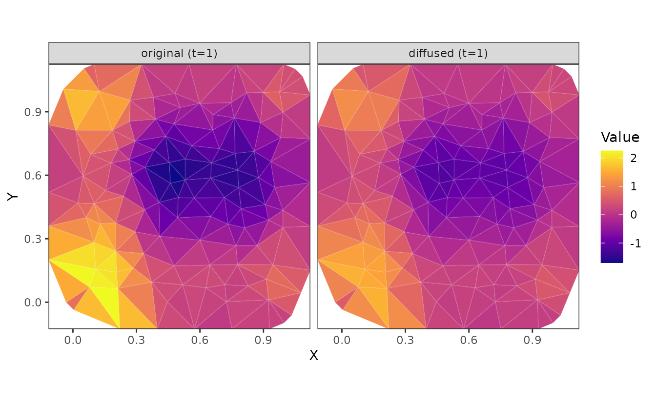

plot_diffused_covariate(fit_st, component = "combined")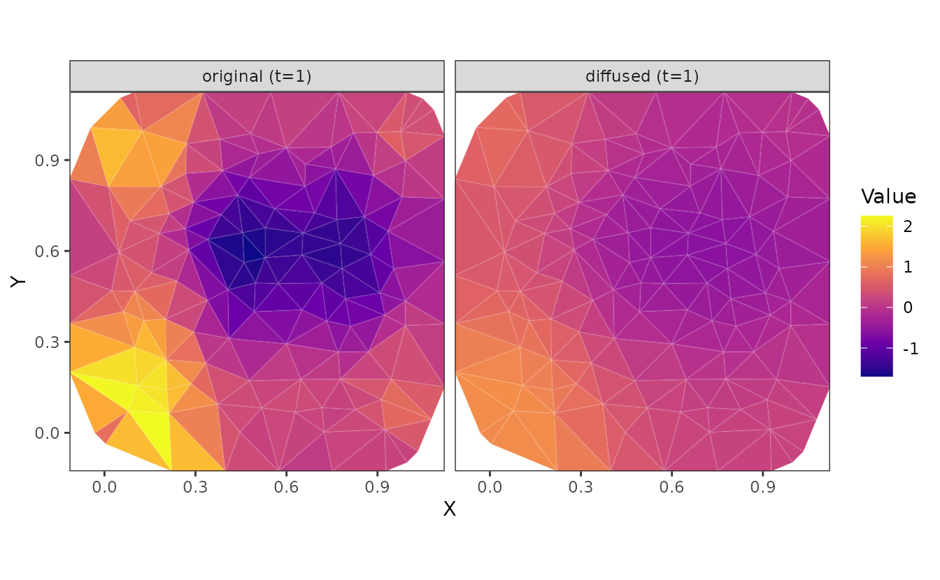

We could also have plotted the spatially diffused covariate at the original locations from the predictions.

pred <- predict(fit_st)

ggplot(pred, aes(X, Y, colour = x1)) + geom_point() +
  scale_colour_gradient2()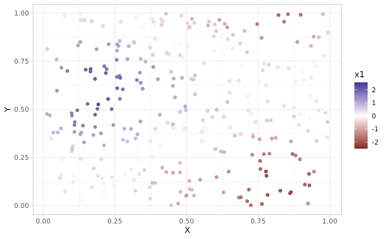


ggplot(pred, aes(X, Y, colour = diffusion_cov_space_x1)) + geom_point() +
  scale_colour_gradient2()

References

Lindmark, M., Anderson, S.C. & Thorson, J.T. (2025). Estimating scale-dependent covariate responses using two-dimensional diffusion derived from the stochastic partial differential equation method. Methods in Ecology and Evolution, 17, 207–218.

Thorson, J., Anderson, S. & Lindmark, M. (2026). Temperature carryover effect revealed for marine fishes using spatio-temporal distributed lag models.

2026-05-22

Simple spatial diffusion example

Space-time example with additive terms

Plot diffusion kernels

References