Create an areal grid domain by overlaying point data

Build or use an sf polygon grid, overlay point observations onto grid cells, construct grid-cell adjacency, and return labelled data plus an sdmTMBareal domain for SAR/CAR models.

Usage

make_areal_grid(
  data,
  xy_cols,
  spatial_domain = NULL,
  cellsize = NULL,
  n = NULL,
  square = TRUE,
  space_column = "grid_cell",
  adjacency = c("rook", "queen"),
  crs = NA
)

Arguments

data

A data frame containing point coordinates.

xy_cols

Character vector of length 2 naming spatial coordinate columns in data.

spatial_domain

Optional sf/sfc polygon object. If cellsize or n is supplied, this object is treated as a boundary from which a grid is generated and clipped. Otherwise it is treated as the grid itself.

cellsize

Optional cell size passed to sf::st_make_grid().

n

Optional grid dimensions passed to sf::st_make_grid(). Ignored if cellsize is supplied.

square

Logical passed to sf::st_make_grid(). Use FALSE for hexagonal grids.

space_column

Column name to add to returned data.

adjacency

Polygon adjacency type: "rook" for shared edges or "queen" for any touching boundary.

crs

Optional coordinate reference system for data coordinates, passed to sf::st_as_sf().

Value

A list with data, grid, and domain elements. domain can be supplied to sdmTMB() via the mesh argument.

See also

make_areal_domain()

Examples

library(ggplot2)

# Basic example of using make_areal_grid()

dat <- data.frame(
  x = c(0.25, 1.25, 0.25, 1.25),
  y = c(0.25, 0.25, 1.25, 1.25),
  depth = c(12, 18, 9, 15)
)

boundary <- sf::st_as_sf(
  sf::st_as_sfc(sf::st_bbox(c(xmin = 0, ymin = 0, xmax = 2, ymax = 2)))
)

areal_grid <- make_areal_grid(
  data = dat,
  xy_cols = c("x", "y"),
  spatial_domain = boundary,
  n = c(2, 2)
)

head(areal_grid$data)
#>      x    y depth grid_cell
#> 1 0.25 0.25    12  cell_001
#> 2 1.25 0.25    18  cell_002
#> 3 0.25 1.25     9  cell_003
#> 4 1.25 1.25    15  cell_004
areal_grid$domain$n_s
#> [1] 4

# Dogfish example going from a data frame to overlaying a grid

# Convert to an sf object:
dogfish_points <- st_as_sf(dogfish, coords = c("X", "Y"), crs = NA)

# make a boundary polygon around observations:
dogfish_boundary <- st_union(dogfish_points) |>
  st_convex_hull() |>
  st_as_sf()

# overlay a grid and create objects for fitting:
dogfish_grid_obj <- make_areal_grid(
  dogfish,
  xy_cols = c("X", "Y"),
  spatial_domain = dogfish_boundary,
  n = c(25L, 20L),
  space_column = "cell_id"
)

names(dogfish_grid_obj)
#> [1] "data"   "grid"   "domain"

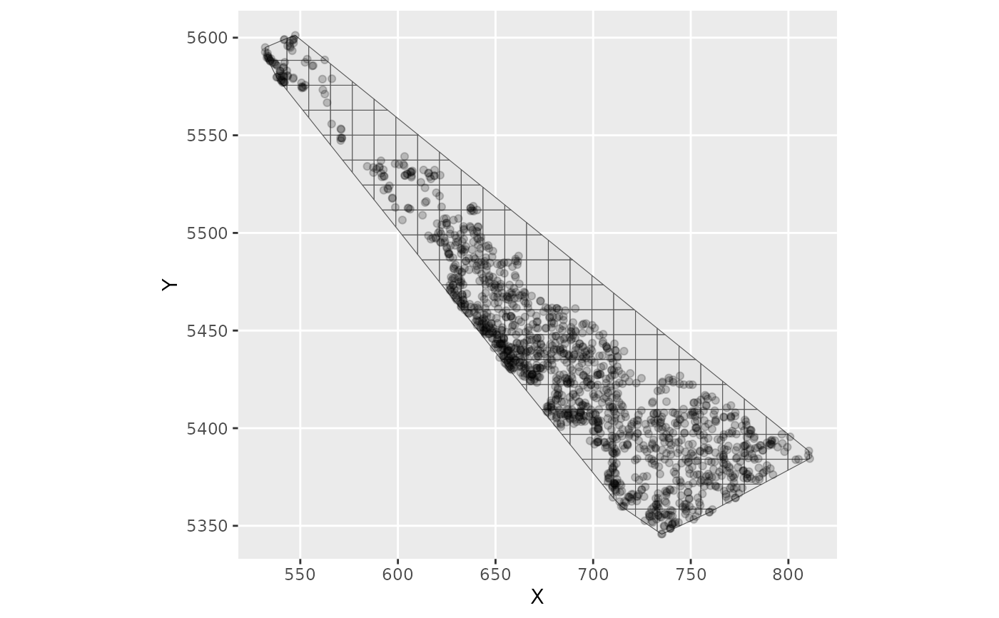
ggplot() + 
  geom_sf(data = dogfish_grid_obj$grid) + 
  geom_point(data = dogfish_grid_obj$data, aes(X, Y), alpha = 0.2)


fit_car <- sdmTMB(
  catch_weight ~ poly(log(depth), 2),
  data = dogfish_grid_obj$data,
  mesh = dogfish_grid_obj$domain,
  spatial_model = "car",
  family = tweedie(link = "log"),
  spatial = "on",
  offset = log(dogfish_grid_obj$data$area_swept)
)
fit_car
#> Spatial model fit by ML ['sdmTMB']
#> Formula: catch_weight ~ poly(log(depth), 2)
#> Mesh: dogfish_grid_obj$domain (isotropic covariance)
#> Data: dogfish_grid_obj$data
#> Family: tweedie(link = 'log')
#>  
#> Conditional model:
#>                      coef.est coef.se
#> (Intercept)              5.32    0.39
#> poly(log(depth), 2)1   -26.20    4.83
#> poly(log(depth), 2)2   -21.92    2.76
#> 
#> Dispersion parameter: 9.03
#> Tweedie p: 1.74
#> CAR spatial dependence: 0.95
#> Spatial CAR field scale: 1.94
#> ML criterion at convergence: 6187.438
#> 
#> See ?tidy.sdmTMB to extract these values as a data frame.