Accounting for hook competition with a censored Poisson • sdmTMB

library(sdmTMB)
library(ggplot2)

Introduction

A longline set has a fixed number of baited hooks. Once most baits have been taken, by the target species, other species, or lost to mechanical failure, fish of the target species have fewer chances to find a baited hook. Catch counts from sets with high bait removal therefore underestimate what would have been caught without hook competition. This bias can differ by year, depending on how many sets were saturated.

Watson et al. (2023) proposed treating catch counts from these sets as right-censored. For a set where the proportion of baits removed reaches a species-specific breakdown point $p^*$ , the observed count $c$ is treated as a lower bound on the count that would have been observed without hook competition. For all other sets, the count is used as usual:

$\Pr(c \mid \mu) = \begin{cases} f(c; \mu), & p < p^* \ \text{(uncensored)},\\ 1 - F(c - 1; \mu), & p \ge p^* \ \text{(right-censored)}, \end{cases}$

where $f$ and $F$ are the Poisson probability mass function and cumulative distribution function and $p$ is the proportion of baits removed. A censored zero has a likelihood of exactly 1, so it contributes no information.

Watson et al. (2023) used simulations to show that this approach recovers relative abundance trends much better than raw CPUE or instantaneous catch rate corrections. It is available in sdmTMB through the censored_poisson() family.

The data

We’ll use the yelloweye dataset that comes with sdmTMB. It contains Yelloweye Rockfish catch counts from the Hard Bottom Longline Survey (South) off the west coast of Vancouver Island, British Columbia. For each set, we know the number of hooks deployed and the number of hooks that came back still baited.

d <- yelloweye
d$prop_removed <- 1 - d$bait_returned / d$hook_count
d$fyear <- as.factor(d$year)
d$log_depth <- log(d$depth)
d$obs_id <- as.factor(seq_len(nrow(d)))
head(d)
#>   year longitude latitude        X        Y catch_count hook_count
#> 1 2007 -128.2567 50.86167 552.3141 5634.705           0        450
#> 2 2007 -128.3450 50.82000 546.1385 5630.013           0        445
#> 3 2007 -128.4433 50.81500 539.2161 5629.400          27        444
#> 4 2007 -128.8383 50.67667 511.4228 5613.882           0        451
#> 5 2007 -128.7433 50.68833 518.1306 5615.199          66        450
#> 6 2007 -128.7617 50.68833 516.8356 5615.194           0        443
#>   bait_returned depth prop_removed fyear log_depth obs_id
#> 1           209  29.2    0.5355556  2007  3.374169      1
#> 2           279  21.9    0.3730337  2007  3.086487      2
#> 3           201  56.6    0.5472973  2007  4.036009      3
#> 4           254 212.1    0.4368071  2007  5.357058      4
#> 5            92 166.4    0.7955556  2007  5.114395      5
#> 6           213 173.7    0.5191874  2007  5.157330      6

In many sets, nearly all baits were removed:

ggplot(d, aes(prop_removed)) +
  geom_histogram(bins = 30) +
  labs(x = "Proportion of baits removed", y = "Number of sets")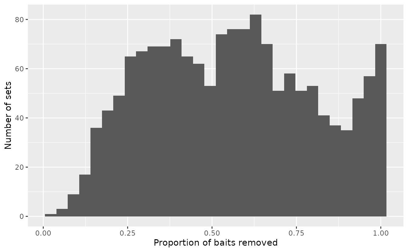

Choosing the breakdown point

Watson et al. (2023) suggest choosing $p^*$ by looking at how mean catch changes as bait removal increases. They fit a smoother of catch against the proportion of baits removed, accounting for year and with log hook count as an offset, and look for where the curve starts to decline. We can do this with mgcv:

library(mgcv)
fit_gam <- gam(
  catch_count ~ s(prop_removed) + fyear + offset(log(hook_count)),
  family = nb(), data = d
)
nd <- data.frame(
  prop_removed = seq(min(d$prop_removed), 1, length.out = 200),
  fyear = d$fyear[1],
  hook_count = 1
)
p <- predict(fit_gam, newdata = nd, se.fit = TRUE)
nd$est <- p$fit
nd$se <- p$se.fit
ggplot(nd, aes(prop_removed, exp(est - max(est)))) +
  geom_ribbon(aes(ymin = exp(est - 2 * se - max(est)),
    ymax = exp(est + 2 * se - max(est))), alpha = 0.3) +
  geom_line() +
  geom_vline(xintercept = 0.85, lty = 2) +
  labs(x = "Proportion of baits removed", y = "Relative mean catch")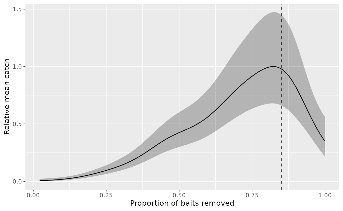

Mean catch rises with bait removal, because sets with more fish remove more baits, until about 0.85. After that it drops, consistent with hook competition. Watson et al. (2023) also chose $p^* = 0.85$ for Yelloweye Rockfish, so we’ll use that value.

pstar <- 0.85
mean(d$prop_removed >= pstar)
#> [1] 0.1565106

About 16% of sets will be treated as censored. The proportion varies by year, and that variation is what biases an uncorrected index:

round(tapply(d$prop_removed >= pstar, d$year, mean), 2)
#> 2007 2009 2011 2014 2016 2018 2020 2022 
#> 0.18 0.08 0.32 0.02 0.11 0.15 0.18 0.21

Fitting the models

We specify censoring with the censored_upper argument in sdmTMBcontrol(). It is a vector with one element per row of data:

a value equal to the observed count means the observation is not censored;
NA means the observation is right-censored with no upper bound;
a value greater than the observed count means the observation is interval-censored between the observed count and that value.

The response is the observed catch count.

upr <- ifelse(d$prop_removed >= pstar, NA, d$catch_count)

We’ll fit a model with year effects, a quadratic effect of log depth, a spatial random field, and an observation-level random intercept, (1 | obs_id). The observation-level intercept makes this a Poisson-lognormal model and accounts for overdispersion, as in Watson et al. (2023). The offset is log hook count, so the index is relative catch per hook.

First, a standard Poisson model that ignores hook competition:

mesh <- make_mesh(d, c("X", "Y"), cutoff = 10)

fit_pois <- sdmTMB(
  catch_count ~ 0 + fyear + poly(log_depth, 2) + (1 | obs_id),
  offset = log(d$hook_count),
  data = d,
  mesh = mesh,
  family = poisson(),
  time = "year",
  spatial = "on",
  spatiotemporal = "off"
)

Now the censored version. We only need to change the family and pass censored_upper:

fit_cens <- update(
  fit_pois,
  family = censored_poisson(),
  control = sdmTMBcontrol(censored_upper = upr)
)
sanity(fit_cens)
fit_cens
#> Spatial model fit by ML ['sdmTMB']
#> Formula: catch_count ~ 0 + fyear + poly(log_depth, 2) + (1 | obs_id)
#> Mesh: sdmTMBmesh (isotropic covariance)
#> Time column: year
#> Data: data.frame
#> Family: censored_poisson(link = 'log')
#>  
#> Random intercepts and/or slopes:
#> 
#> Conditional model:
#>      Groups        Name    Variance    Std.Dev. 
#>      obs_id (Intercept)        2.37        1.54 
#> 
#> Conditional model:
#>                     coef.est coef.se
#> fyear2007              -4.66    0.79
#> fyear2009              -5.03    0.78
#> fyear2011              -4.32    0.77
#> fyear2014              -5.47    0.78
#> fyear2016              -5.51    0.78
#> fyear2018              -4.78    0.79
#> fyear2020              -5.14    0.78
#> fyear2022              -4.77    0.78
#> poly(log_depth, 2)1   -12.33    4.33
#> poly(log_depth, 2)2   -28.19    3.26
#> 
#> Matérn range: 60.04
#> Spatial SD: 2.97
#> ML criterion at convergence: 4235.762
#> 
#> See ?tidy.sdmTMB to extract these values as a data frame.

Adding an upper bound

When many observations are censored and the data are limited, the right-censored model may not converge. Watson et al. (2023) describe an optional upper bound on the censored counts (their Supplementary Material S.3), turning right-censored observations into interval-censored ones. The bound adds the expected number of target-species catches “missed” because of hook competition, based on the number of hooks emptied past the breakdown point. The function get_censored_upper() calculates this bound:

upr_bounded <- get_censored_upper(
  prop_removed = d$prop_removed,
  n_catch = d$catch_count,
  n_hooks = d$hook_count,
  pstar = pstar
)
fit_cens_bounded <- update(
  fit_pois,
  family = censored_poisson(),
  control = sdmTMBcontrol(censored_upper = upr_bounded)
)

Watson et al. (2023) also suggest treating the largest catch counts each year as uncensored, regardless of bait removal, to help convergence. To do that, set censored_upper equal to catch_count for those rows.

Comparing indices

We’ll predict over the survey grid hbll_s_grid and calculate an index for each model. We set the offset to 0 for prediction (i.e., one hook) and leave out the observation-level random intercepts with re_form_iid = NA. The grid contains depths outside the sampled range, so we clamp depth to the range of the data so that the quadratic is not extrapolated.

grid <- replicate_df(hbll_s_grid, "year", unique(d$year))
grid$fyear <- as.factor(grid$year)
grid$log_depth <- log(pmin(pmax(grid$depth, min(d$depth)), max(d$depth)))

get_ind <- function(fit, label) {
  ind <- get_index(
    fit, newdata = grid, offset = rep(0, nrow(grid)),
    predict_args = list(re_form_iid = NA),
    bias_correct = TRUE
  )
  ind$model <- label
  ind
}
ind <- rbind(
  get_ind(fit_pois, "Poisson"),
  get_ind(fit_cens, "Censored Poisson"),
  get_ind(fit_cens_bounded, "Censored Poisson (upper bound)")
)

Since these are relative indices, we’ll scale each by its geometric mean before plotting:

ind <- do.call(rbind, lapply(split(ind, ind$model), function(x) {
  gm <- exp(mean(log(x$est)))
  x[, c("est", "lwr", "upr")] <- x[, c("est", "lwr", "upr")] / gm
  x
}))
ggplot(ind, aes(year, est, colour = model, fill = model)) +
  geom_ribbon(aes(ymin = lwr, ymax = upr), alpha = 0.15, colour = NA) +
  geom_line() +
  geom_point() +
  labs(x = "Year", y = "Relative index", colour = NULL, fill = NULL) +
  theme(legend.position = "bottom")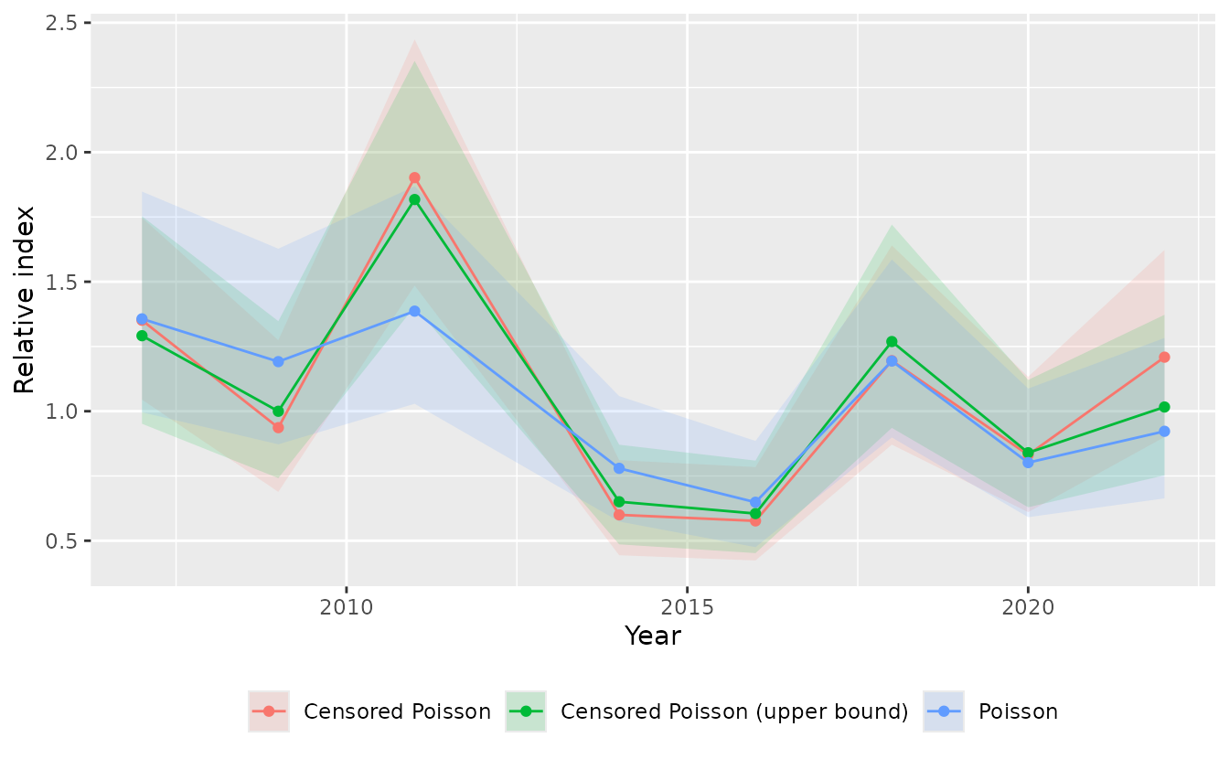

The censored models differ most from the uncensored Poisson model in years with an unusually high or low proportion of censored sets. For example, 2011 had the highest proportion of saturated sets, and its index is higher once we account for hook competition. 2014 had very few saturated sets, and its index is lower relative to the other years. Here, the upper bound mostly has a modest effect, pulling some years (e.g., 2022) partway back towards the Poisson estimates by limiting how large the censored counts can be.

Summary

Calculate the proportion of baits removed for each set.
Choose a breakdown point $p^*$ , e.g., by plotting a smoother of catch against bait removal.
Build a censored_upper vector: the observed count for uncensored sets and NA (or an upper bound) for sets at or above $p^*$ .
Fit with family = censored_poisson() and control = sdmTMBcontrol(censored_upper = ...), ideally with an observation-level random intercept to account for overdispersion.

See Watson et al. (2023) for the full method, simulation tests, and an application to 11 species.

References

Watson, J., Edwards, A.M. & Auger-Méthé, M. (2023). A statistical censoring approach accounts for hook competition in abundance indices from longline surveys. Canadian Journal of Fisheries and Aquatic Sciences, 80, 468–486.