
Fit a spatial or spatiotemporal generalized linear mixed effects model (GLMM) with TMB (Template Model Builder), by default through the RTMB package. Spatial and spatiotemporal Gaussian random fields are approximated with the SPDE (stochastic partial differential equation) approach, which represents them as Gaussian Markov random fields on a mesh. This allows for efficient modelling of data that are correlated in space and/or time. Areal spatial and spatiotemporal models (simultaneous or conditional autoregressive; SAR or CAR) are also available. See the model description vignette for details.
Usage
sdmTMB(
  formula,
  data,
  mesh,
  time = NULL,
  family = gaussian(link = "identity"),
  spatial = c("on", "off"),
  spatiotemporal = c("iid", "ar1", "rw", "off"),
  extra_time = NULL,
  spatial_model = c("spde", "sar", "car"),
  share_range = TRUE,
  anisotropy = FALSE,
  offset = NULL,
  weights = NULL,
  dispformula = ~1,
  censored_upper = NULL,
  distribution_column = NULL,
  spatial_varying = NULL,
  time_varying = NULL,
  time_varying_type = c("rw", "rw0", "ar1"),
  nonlocal_formula = NULL,
  nonlocal_data = NULL,
  knots = NULL,
  reml = FALSE,
  priors = sdmTMBpriors(),
  bayesian = FALSE,
  control = sdmTMBcontrol(),
  previous_fit = NULL,
  silent = TRUE,
  do_fit = TRUE,
  do_index = FALSE,
  predict_args = NULL,
  index_args = NULL,
  experimental = NULL
)
Arguments
- formula
A model formula. Random intercepts and slopes use lme4 syntax, e.g.,
(1 | g),(0 + depth | g), or(1 + depth | g), wheregis a character or factor column. As in lme4, intercepts and slopes within a term are correlated. Penalized smooths use mgcv syntax, e.g.,s(depth), and threshold terms usebreakpt()orlogistic(). For delta models, optionally a list of two formulas. See Details.- data
A data frame. Rows with missing values in the response or any variable the model uses (including
weightsandoffset) are omitted before fitting, as withna.action = na.omitinstats::glm(). The rows used are stored in the returned object asdata.- mesh
An object from
make_mesh()forspatial_model = "spde"or frommake_areal_domain()for"sar"or"car".- time
An optional time column name (as character). Can be left as
NULLfor a model with only spatial random fields; however, if the data are actually spatiotemporal and you wish to calculate derived quantities downstream (e.g.,get_index()orget_cog()), then supply the time argument.- family
A family object specifying the response distribution and link:
gaussian(),Gamma(),binomial(),poisson(), or one of the additional families listed in Families (e.g.,tweedie(),nbinom2(),delta_gamma()). See 'Binomial families', 'Censored families', and 'Delta/hurdle models' in Details. Experimental multi-family models take a named list of families;distribution_columnthen assigns each row to one of them. See the multi-family vignette for supported combinations.- spatial
Estimate spatial random fields? Options are
'on'/'off'or equivalentlyTRUE/FALSE. Optionally, a list for delta models, e.g.list('on', 'off').- spatiotemporal
Estimate the spatiotemporal random fields as
'iid'(independent and identically distributed; default), stationary'ar1'(first-order autoregressive), a random walk ('rw'), or fixed at 0'off'. Will be set to'off'iftime = NULL. If a delta model, can be a list. E.g.,list('off', 'ar1'). Guidance: Use'iid'if spatiotemporal correlation is negligible or already accounted for in fixed effects;'ar1'if correlation between consecutive time steps decays gradually;'rw'if changes between time steps are cumulative (each step builds on the last). If the AR1 correlation coefficient (rho) is estimated close to 1 (say > 0.99), consider switching to'rw'. See the model description vignette for mathematical details. Capitalization is ignored.TRUEgets converted to'iid'andFALSEgets converted to'off'.- extra_time
Optional extra time slices (e.g., years) to include for interpolation or forecasting with the predict function. See the Details section below.
- spatial_model
Spatial process model.
"spde"uses the default continuous-space SPDE approximation."sar"and"car"use areal spatial autoregressive models with an areal domain supplied tomesh. Capitalization is ignored.Logical: estimate a single range parameter shared by the spatial and spatiotemporal fields (
TRUE, default) or separate range parameters (FALSE)? For delta models, can be a list, e.g.,list(TRUE, FALSE). Applies to SPDE models only.- anisotropy
Logical: allow for anisotropy (spatial correlation that is directionally dependent)? See
plot_anisotropy(). Applies to SPDE models only and is shared by both components of a delta model.- offset
A numeric vector representing the model offset or a character value representing the column name of the offset. In delta/hurdle models, this applies only to the positive component except for Poisson-link delta models, where it also enters the occurrence-probability calculation. Usually a log transformed variable.
- weights
An optional numeric vector (not a column name) of weights on each observation's contribution to the likelihood. As in glmmTMB, weights need not sum to one and are not rescaled. For binomial-type families with a proportion response,
weightsgives the number of trials instead; see 'Binomial families' in Details.- dispformula
A one-sided formula for the dispersion parameter (e.g.,
phi). The default,~ 1, estimates a single value. Ignored for families without a dispersion parameter (e.g., binomial or Poisson). In delta models, applies to the positive component. Not yet available for multi-family models or truncated negative binomial families.- censored_upper
Upper bounds for the censored families (see Families): a numeric vector or the name of a column in
data. Each response is a count between its observed value and this bound. A bound equal to the response is uncensored, a larger bound is interval-censored, andInfis right-censored (capped at the number of trials forcensored_binomial()andcensored_betabinomial()). Non-integer bounds are rounded down. For left censoring (e.g., fewer than 5), use a response of 0 and a bound of 4.- distribution_column
For experimental multi-family models, the name of the column in
datamapping each row to a family in the namedfamilylist. See the multi-family vignette for the supported family and method combinations.- spatial_varying
An optional one-sided formula of coefficients that should vary in space as random fields. Allows the effect of a covariate to differ spatially. You likely want to include the same variable as a fixed effect in
formulato estimate the average effect—the spatial field then represents deviations from that average. For example, useformula = y ~ depthandspatial_varying = ~ 0 + depthto model an average depth effect plus spatially varying deviations. If a (scaled) time column is used, this creates a local-time-trend model. See doi:10.1111/ecog.05176 and the spatial trends vignette. Predictors should usually be centered to have mean zero and standard deviation approximately 1. The spatial intercept is controlled by thespatialargument; setspatial = 'on'or'off'to include or exclude it. For a factor,~ 0 + fgives every level its own field, which would duplicate the spatial intercept field, so setspatial = 'off'to match. Structure is shared in delta models.- time_varying
An optional one-sided formula of coefficients that vary through time following the process set by
time_varying_type. Whether the same covariates should also appear informuladepends on that type. Shared by both components of a delta model.- time_varying_type
The process for
time_varyingcoefficients:'rw'(default): a random walk with the first value estimated freely. Do not also include these covariates informula, or the model is not identifiable; e.g., withtime_varying = ~ 1, useformula = y ~ 0 + ....'rw0': a random walk whose first value has a mean-zero normal prior.'ar1': a stationary first-order autoregressive process with mean zero.
For
'rw0'and'ar1', include the same covariates informula; the time-varying process then describes deviations from that average effect. Shared by both components of a delta model.- nonlocal_formula
An optional one-sided formula of non-local covariate effects:
diffusion()for an effect of conditions in the surrounding area, andtime_lag()for an effect of conditions in previous time steps, e.g.,~ diffusion(x) + time_lag(x). Using both on the same covariate gives one combined effect that spreads over both space and time; different covariates give separate effects. Seetime_lag()for how the lag starts (start). IftimeisNULL, a spatial-only covariate is held constant across time slices. See the non-local covariates vignette, which also explains the reported diffusion scales (MSDK and RMSDK).- nonlocal_data
An optional data frame supplying the
nonlocal_formulacovariate(s) at a different resolution and/or coverage thandata(e.g., a finer grid, or one spanningextra_timeslices). Must contain the meshxy_cols, the diffusion covariate columns, and thetimecolumn ifnonlocal_formulais time-indexed (time_lag()terms, ordiffusion()terms withtimespecified). In that case, it must cover every fitted (+extra_time) time slice. Defaults toNULL, in which casedatais used.- knots
Optional named list containing knot values to be used for basis construction of smoothing terms. See
mgcv::gam()andmgcv::gamm(). E.g.,s(x, bs = 'cc', k = 4), knots = list(x = c(1, 2, 3, 4))- reml
Logical: use REML (restricted maximum likelihood) estimation rather than maximum likelihood? REML accounts for uncertainty in estimating fixed effects and can reduce bias in variance parameter estimates, but prevents likelihood-based model comparison (e.g., AIC) between models with different fixed effects. Use
TRUEif your focus is on random effect variance parameters; useFALSE(default) if comparing models with different fixed effects or performing index standardization.- priors
Optional penalties/priors via
sdmTMBpriors(). Must currently be shared across delta models.- bayesian
Logical indicating if the model will be passed to tmbstan. If
TRUE, Jacobian adjustments are applied to account for parameter transformations when priors are applied.- control
Optimization control options via
sdmTMBcontrol().- previous_fit
A previously fitted sdmTMB model to initialize the optimization with. Can greatly speed up fitting. Note that the model must be set up exactly the same way. However, the data and
weightsarguments can change, which can be useful for cross-validation.- silent
Silent or include optimization details? Helpful to set to
FALSEfor models that take a while to fit.- do_fit
Fit the model (
TRUE) or return the processed data without fitting (FALSE)?- do_index
![[Deprecated]](figures/lifecycle-deprecated.svg) Do index
standardization calculations while fitting? Instead, fit the model and
then pass the fitted model and
Do index
standardization calculations while fitting? Instead, fit the model and
then pass the fitted model and newdatadirectly toget_index(),get_cog(),get_eao(), orget_weighted_average(). IfTRUE, thenpredict_argsmust have anewdataelement supplied andareacan be supplied toindex_args.- predict_args
- A list of arguments
to pass to
predict.sdmTMB()ifdo_index = TRUE. - index_args
- A list of arguments to
pass to
get_index()ifdo_index = TRUE. Currently,areaandderived_linkare supported. - experimental
A named list for esoteric or in-development options. Here be dragons.
Value
An object (list) of class sdmTMB. Useful elements include:
model: output fromstats::nlminb()sd_report: output fromTMB::sdreport()orRTMB::sdreport()gradients: gradients of the marginal log likelihood with respect to each fixed effectdata: the data used in fitting (rows with missing values removed)spde: the object supplied tomeshfamily: the family object, including the inverse link functionfamily$linkinv()backend:"rtmb"or"tmb"; seesdmTMBcontrol()tmb_obj: the objective function object fromTMB::MakeADFun()orRTMB::MakeADFun()tmb_data,tmb_params,tmb_map: the data, parameter, and map lists passed toMakeADFun()
Details
Model description
sdmTMB fits GLMMs with spatial and/or spatiotemporal random fields, which account for correlation in the data due to spatial proximity, or alternatively, latent spatial and spatiotemporal effects. Spatial fields represent consistent spatial patterns, while spatiotemporal fields represent spatial patterns that vary over time. See the model description vignette for mathematical details and the paper: doi:10.18637/jss.v115.i02
Binomial families
Following the structure of stats::glm() and glmmTMB, a binomial
family can be specified in one of four ways: (1) the response may be a factor
(success is interpreted as any level other than the first level), (2) the
response may be binary (0/1), (3) the response can be a matrix of form
cbind(success, failure), and (4) the response may be observed
proportions, and the weights argument is used to specify the binomial size
(N) parameter (prob ~ ..., weights = N).
Smooth terms
Smooth terms can be included following GAMs (generalized additive models)
using + s(x), which implements a smooth from mgcv::s(). sdmTMB uses
penalized smooths, constructed via mgcv::smooth2random(). This is a similar
approach implemented in gamm4 and brms, among other packages.
Within these smooths, the same syntax commonly used in mgcv::s() or
mgcv::t2() can be applied, e.g. 2-dimensional smooths may be constructed
with + s(x, y) or + t2(x, y); smooths can be specific to various factor
levels, + s(x, by = group); the basis function dimensions may be specified,
e.g. + s(x, k = 4); and various types of splines may be constructed such as
cyclic splines to model seasonality (perhaps with the knots argument also
supplied).
Threshold models
A linear break-point relationship for a covariate can be included via
+ breakpt(variable) in the formula, where variable is a single covariate
corresponding to a column in data. In this case, the relationship is linear
up to a point and then constant (hockey-stick shaped).
Similarly, a logistic-function threshold model can be included via
+ logistic(variable). This option models the relationship as a logistic
function of the 50% and 95% values. This is similar to length- or size-based
selectivity in fisheries, and is parameterized by the points at which f(x) =
0.5 or 0.95. See the
threshold vignette.
Note that only a single threshold covariate can be included. For delta
families, the threshold applies to both components, and threshold terms are
not available if formula is a list.
Extra time: forecasting or interpolating
Extra time slices (e.g., years) can be included for interpolation or
forecasting with the predict function via the extra_time argument. The
predict function requires all time slices to be defined when fitting the
model to ensure the various time indices are set up correctly. Be careful if
including extra time slices that the model remains identifiable. For example,
including + as.factor(year) in formula will render a model with no data
to inform the expected value in a missing year. sdmTMB() makes no attempt
to determine if the model makes sense for forecasting or interpolation. The
options time_varying, spatiotemporal = "rw", spatiotemporal = "ar1",
or a smoother on the time column provide mechanisms to predict over missing
time slices; time_varying and spatiotemporal random-walk or AR(1) fields
include process error.
extra_time can also be used to fill in missing time steps for the purposes
of a random walk or AR(1) process if the gaps between time steps are uneven.
extra_time can include only extra time steps or all time steps including
those found in the fitted data. This latter option may be simpler.
Regularization and priors
You can achieve regularization via penalties (priors) on the fixed effect
parameters. See sdmTMBpriors(). You can fit the model once without
penalties and look at the output of print(your_model) or tidy(your_model)
or fit the model with do_fit = FALSE and inspect
head(your_model$tmb_data$X_ij[[1]]) if you want to see how the formula is
translated to the fixed effect model matrix. Also see the
Bayesian vignette.
Delta/hurdle models
Delta models (also known as hurdle models) can be fit as two separate models
or at the same time by using an appropriate delta family (see the list under
family). Delta families with type = "poisson-link" use a Poisson-link
parameterization instead of a classic hurdle model; see the Poisson-link vignette.
If fit with a delta family, by default the formula, spatial, and spatiotemporal
components are shared. Some elements can be specified independently for the two models
using a list format. These include formula, spatial, spatiotemporal,
and share_range. The first element of the list is for the binomial component
and the second element is for the positive component (e.g., Gamma).
Other elements must be shared for now (e.g., spatially varying coefficients,
time-varying coefficients), and dispformula applies to the positive
component only. Furthermore, there are currently limitations if
specifying two formulas as a list: smoothers and random effect terms must
be identical between the two formulas, and threshold effects must be
specified through a single formula that is shared across the two models.
The main advantage of specifying such models using a delta family (compared
to fitting two separate models) is (1) coding simplicity and (2) calculation
of uncertainty on derived quantities such as an index of abundance with
get_index() using the generalized delta method within TMB. Also, selected
parameters can be shared across the models.
See the delta-model vignette.
Censored families
Censored families treat some observations as known only to lie within a
range, e.g., catch counts on longlines where competition for hooks hides
the true number caught. Supply the bounds with censored_upper. All but
censored_poisson() need the RTMB backend (the default). See Families
and the hook competition vignette.
Areal models
For data on areal units (e.g., grid cells or management areas) rather than
point locations, build a domain with make_areal_domain(), pass it to
mesh, and set spatial_model = "sar" or "car". share_range and
anisotropy do not apply. See the areal model vignette.
Index standardization
For index standardization, you may wish to include 0 + as.factor(year)
(or whatever the time column is called) in the formula. See a basic
example of index standardization in the relevant
package vignette.
You will need to specify the time argument. See get_index().
References
Main reference introducing the package to cite when using sdmTMB:
Anderson, S.C., E.J. Ward, P.A. English, L.A.K. Barnett, J.T. Thorson. 2025. sdmTMB: an R package for fast, flexible, and user-friendly generalized linear mixed effects models with spatial and spatiotemporal random fields. Journal of Statistical Software. 115(2):1–46. doi:10.18637/jss.v115.i02 .
Reference for local trends:
Barnett, L.A.K., E.J. Ward, S.C. Anderson. 2021. Improving estimates of species distribution change by incorporating local trends. Ecography. 44(3):427-439. doi:10.1111/ecog.05176 .
Further explanation of the model and application to calculating climate velocities:
English, P., E.J. Ward, C.N. Rooper, R.E. Forrest, L.A. Rogers, K.L. Hunter, A.M. Edwards, B.M. Connors, S.C. Anderson. 2022. Contrasting climate velocity impacts in warm and cool locations show that effects of marine warming are worse in already warmer temperate waters. Fish and Fisheries. 23(1) 239-255. doi:10.1111/faf.12613 .
Discussion of and illustration of some decision points when fitting these models:
Commander, C.J.C., L.A.K. Barnett, E.J. Ward, S.C. Anderson, T.E. Essington. 2022. The shadow model: how and why small choices in spatially explicit species distribution models affect predictions. PeerJ 10: e12783. doi:10.7717/peerj.12783 .
Application and description of threshold/break-point models:
Essington, T.E., S.C. Anderson, L.A.K. Barnett, H.M. Berger, S.A. Siedlecki, E.J. Ward. 2022. Advancing statistical models to reveal the effect of dissolved oxygen on the spatial distribution of marine taxa using thresholds and a physiologically based index. Ecography. 2022: e06249 doi:10.1111/ecog.06249 .
Application to fish body condition:
Lindmark, M., S.C. Anderson, M. Gogina, M. Casini. 2023. Evaluating drivers of spatiotemporal variability in individual condition of a bottom-associated marine fish, Atlantic cod (Gadus morhua). ICES Journal of Marine Science. 80(5): 1539–1550.
Non-local covariates:
Lindmark, M., Anderson, S.C., and Thorson, J.T. 2026. Estimating scale-dependent covariate responses using two-dimensional diffusion derived from the stochastic partial differential equation method. Methods in Ecology and Evolution 17: 207–218. doi:10.1111/2041-210X.70177 .
Thorson, J.T., Anderson, S.C., and Lindmark, M. 2026. Temperature carryover effect revealed for marine fishes using spatio-temporal distributed lag models. EcoEvoRxiv. doi:10.32942/X2W95P .
Several sections of the original TMB model code were adapted from the VAST R package:
Thorson, J.T. 2019. Guidance for decisions using the Vector Autoregressive Spatio-Temporal (VAST) package in stock, ecosystem, habitat and climate assessments. Fish. Res. 210:143–161. doi:10.1016/j.fishres.2018.10.013 .
Code for the family R-to-TMB implementation, selected parameterizations of
the observation likelihoods, general package structure inspiration, and the
idea behind the TMB prediction approach were adapted from the glmmTMB R
package:
Brooks, M.E., K. Kristensen, K.J. van Benthem, A. Magnusson, C.W. Berg, A. Nielsen, H.J. Skaug, M. Maechler, B.M. Bolker. 2017. glmmTMB Balances Speed and Flexibility Among Packages for Zero-inflated Generalized Linear Mixed Modeling. The R Journal, 9(2):378-400. doi:10.32614/rj-2017-066 .
Implementation of geometric anisotropy with the SPDE and use of random field GLMMs for index standardization:
Thorson, J.T., A.O. Shelton, E.J. Ward, H.J. Skaug. 2015. Geostatistical delta-generalized linear mixed models improve precision for estimated abundance indices for West Coast groundfishes. ICES J. Mar. Sci. 72(5): 1297–1310. doi:10.1093/icesjms/fsu243 .
Examples
library(sdmTMB)
# Build a mesh to implement the SPDE approach:
mesh <- make_mesh(pcod_2011, c("X", "Y"), cutoff = 20)
# - this example uses a fairly coarse mesh so these examples run quickly
# - 'cutoff' is the minimum distance between mesh vertices in units of the
# x and y coordinates
# - 'cutoff = 10' might make more sense in applied situations for this dataset
# - or build any mesh in 'fmesher' and pass it to the 'mesh' argument in make_mesh()
# - the mesh is not needed if you will be turning off all
# spatial/spatiotemporal random fields
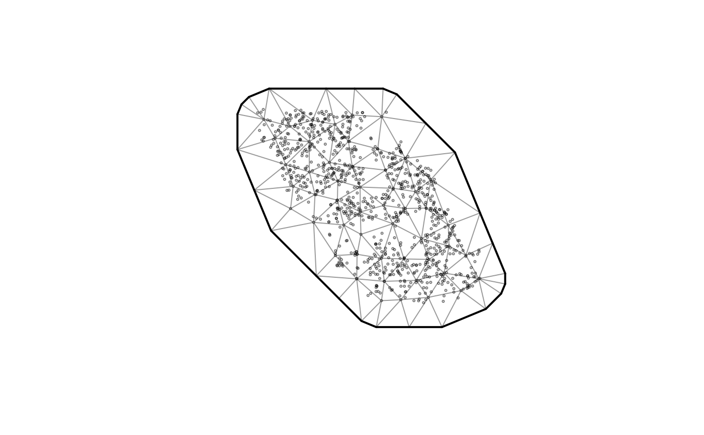
# Quick mesh plot:
plot(mesh)
 # Fit a Tweedie spatial random field GLMM with a smoother for depth:
fit <- sdmTMB(
density ~ s(depth),
data = pcod_2011, mesh = mesh,
family = tweedie(link = "log")
)
fit
#> Spatial model fit by ML ['sdmTMB']
#> Formula: density ~ s(depth)
#> Mesh: mesh (isotropic covariance)
#> Data: pcod_2011
#> Family: tweedie(link = 'log')
#>
#> Conditional model:
#> coef.est coef.se
#> (Intercept) 2.16 0.34
#> sdepth 1.94 3.13
#>
#> Smooth terms:
#> Std. Dev.
#> sd__s(depth) 13.07
#>
#> Dispersion parameter: 13.68
#> Tweedie p: 1.58
#> Matérn range: 16.84
#> Spatial SD: 2.20
#> ML criterion at convergence: 2937.789
#>
#> See ?tidy.sdmTMB to extract these values as a data frame.
# Extract coefficients:
tidy(fit, conf.int = TRUE)
#> # A tibble: 2 × 5
#> term estimate std.error conf.low conf.high
#> <chr> <dbl> <dbl> <dbl> <dbl>
#> 1 (Intercept) 2.16 0.340 1.50 2.83
#> 2 sdepth 1.94 3.13 -4.19 8.07
tidy(fit, effects = "ran_par", conf.int = TRUE)
#> # A tibble: 5 × 5
#> term estimate std.error conf.low conf.high
#> <chr> <dbl> <dbl> <dbl> <dbl>
#> 1 range 16.8 13.7 3.40 83.3
#> 2 phi 13.7 0.663 12.4 15.0
#> 3 sigma_O 2.20 1.23 0.735 6.59
#> 4 tweedie_p 1.58 0.0153 1.55 1.61
#> 5 sd__s(depth) 13.1 NA 6.07 28.2
# Perform several 'sanity' checks:
sanity(fit)
#> ✔ Non-linear minimizer suggests successful convergence
#> ✔ Hessian matrix is positive definite
#> ✔ No extreme or very small eigenvalues detected
#> ✔ No gradients with respect to fixed effects are >= 0.001
#> ✔ No fixed-effect standard errors are NA
#> ✔ No standard errors look unreasonably large
#> ✔ No sigma parameters are < 0.01
#> ✔ No sigma parameters are > 100
#> ✔ Range parameter doesn't look unreasonably large
# Predict on the fitted data; see ?predict.sdmTMB
p <- predict(fit)
# Predict on new data:
p <- predict(fit, newdata = qcs_grid)
head(p)
#> X Y depth depth_scaled depth_scaled2 est est_non_rf est_rf
#> 1 456 5636 347.0834 1.5608122 2.43613479 -4.726638 -4.567385 -0.15925308
#> 2 458 5636 223.3348 0.5697699 0.32463771 2.342470 2.368314 -0.02584421
#> 3 460 5636 203.7408 0.3633693 0.13203724 3.087513 2.979948 0.10756466
#> 4 462 5636 183.2987 0.1257046 0.01580166 3.878560 3.637586 0.24097353
#> 5 464 5636 182.9998 0.1220368 0.01489297 4.020914 3.646532 0.37438240
#> 6 466 5636 186.3892 0.1632882 0.02666303 4.050895 3.543104 0.50779127
#> omega_s
#> 1 -0.15925308
#> 2 -0.02584421
#> 3 0.10756466
#> 4 0.24097353
#> 5 0.37438240
#> 6 0.50779127
# \donttest{
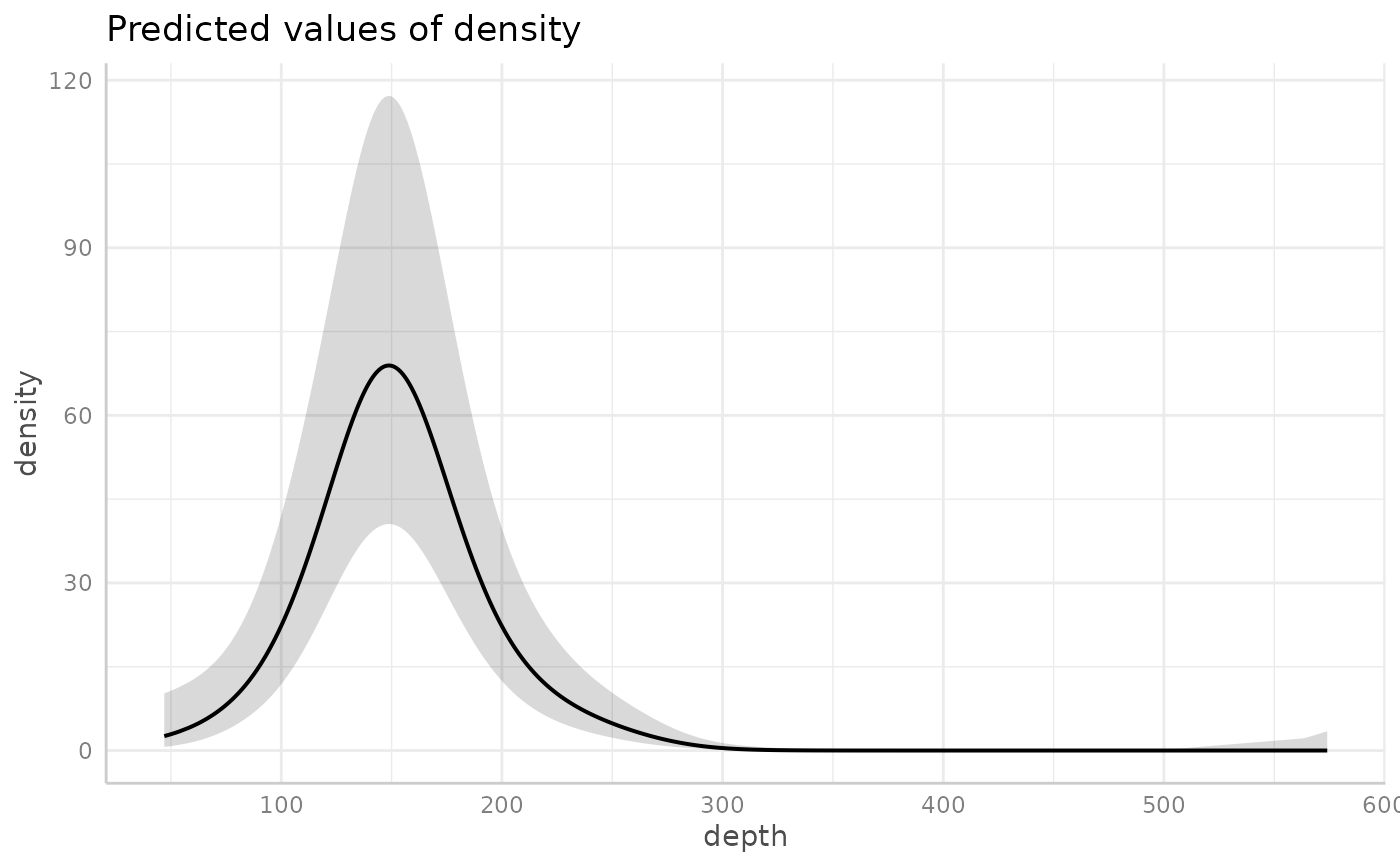
# Visualize the depth effect with ggeffects:
ggeffects::ggpredict(fit, "depth [all]") |> plot()
# Fit a Tweedie spatial random field GLMM with a smoother for depth:
fit <- sdmTMB(
density ~ s(depth),
data = pcod_2011, mesh = mesh,
family = tweedie(link = "log")
)
fit
#> Spatial model fit by ML ['sdmTMB']
#> Formula: density ~ s(depth)
#> Mesh: mesh (isotropic covariance)
#> Data: pcod_2011
#> Family: tweedie(link = 'log')
#>
#> Conditional model:
#> coef.est coef.se
#> (Intercept) 2.16 0.34
#> sdepth 1.94 3.13
#>
#> Smooth terms:
#> Std. Dev.
#> sd__s(depth) 13.07
#>
#> Dispersion parameter: 13.68
#> Tweedie p: 1.58
#> Matérn range: 16.84
#> Spatial SD: 2.20
#> ML criterion at convergence: 2937.789
#>
#> See ?tidy.sdmTMB to extract these values as a data frame.
# Extract coefficients:
tidy(fit, conf.int = TRUE)
#> # A tibble: 2 × 5
#> term estimate std.error conf.low conf.high
#> <chr> <dbl> <dbl> <dbl> <dbl>
#> 1 (Intercept) 2.16 0.340 1.50 2.83
#> 2 sdepth 1.94 3.13 -4.19 8.07
tidy(fit, effects = "ran_par", conf.int = TRUE)
#> # A tibble: 5 × 5
#> term estimate std.error conf.low conf.high
#> <chr> <dbl> <dbl> <dbl> <dbl>
#> 1 range 16.8 13.7 3.40 83.3
#> 2 phi 13.7 0.663 12.4 15.0
#> 3 sigma_O 2.20 1.23 0.735 6.59
#> 4 tweedie_p 1.58 0.0153 1.55 1.61
#> 5 sd__s(depth) 13.1 NA 6.07 28.2
# Perform several 'sanity' checks:
sanity(fit)
#> ✔ Non-linear minimizer suggests successful convergence
#> ✔ Hessian matrix is positive definite
#> ✔ No extreme or very small eigenvalues detected
#> ✔ No gradients with respect to fixed effects are >= 0.001
#> ✔ No fixed-effect standard errors are NA
#> ✔ No standard errors look unreasonably large
#> ✔ No sigma parameters are < 0.01
#> ✔ No sigma parameters are > 100
#> ✔ Range parameter doesn't look unreasonably large
# Predict on the fitted data; see ?predict.sdmTMB
p <- predict(fit)
# Predict on new data:
p <- predict(fit, newdata = qcs_grid)
head(p)
#> X Y depth depth_scaled depth_scaled2 est est_non_rf est_rf
#> 1 456 5636 347.0834 1.5608122 2.43613479 -4.726638 -4.567385 -0.15925308
#> 2 458 5636 223.3348 0.5697699 0.32463771 2.342470 2.368314 -0.02584421
#> 3 460 5636 203.7408 0.3633693 0.13203724 3.087513 2.979948 0.10756466
#> 4 462 5636 183.2987 0.1257046 0.01580166 3.878560 3.637586 0.24097353
#> 5 464 5636 182.9998 0.1220368 0.01489297 4.020914 3.646532 0.37438240
#> 6 466 5636 186.3892 0.1632882 0.02666303 4.050895 3.543104 0.50779127
#> omega_s
#> 1 -0.15925308
#> 2 -0.02584421
#> 3 0.10756466
#> 4 0.24097353
#> 5 0.37438240
#> 6 0.50779127
# \donttest{
# Visualize the depth effect with ggeffects:
ggeffects::ggpredict(fit, "depth [all]") |> plot()
 # Visualize depth effect with visreg: (see ?visreg_delta)
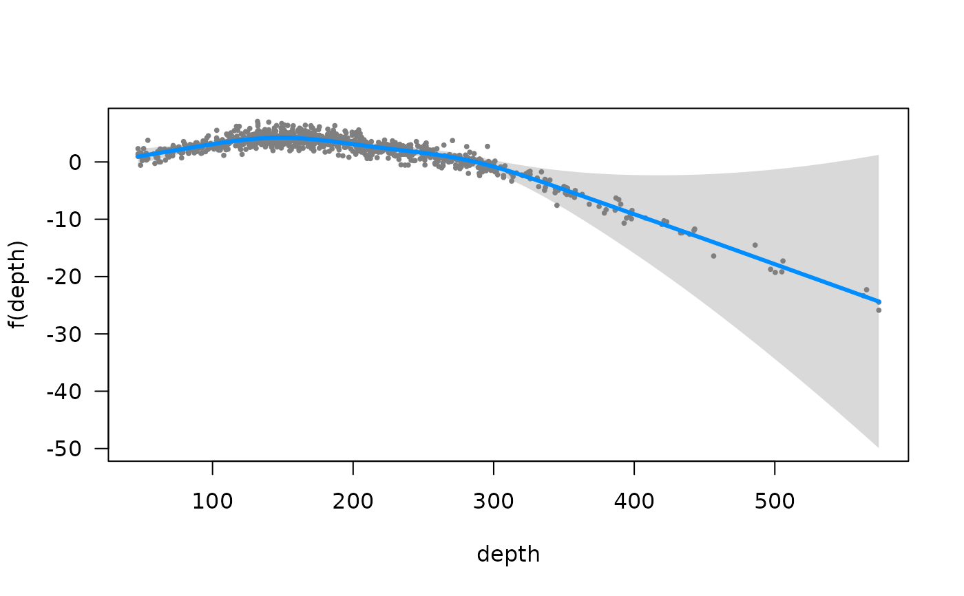
visreg::visreg(fit, xvar = "depth") # link space; randomized quantile residuals
# Visualize depth effect with visreg: (see ?visreg_delta)
visreg::visreg(fit, xvar = "depth") # link space; randomized quantile residuals
 visreg::visreg(fit, xvar = "depth", scale = "response")
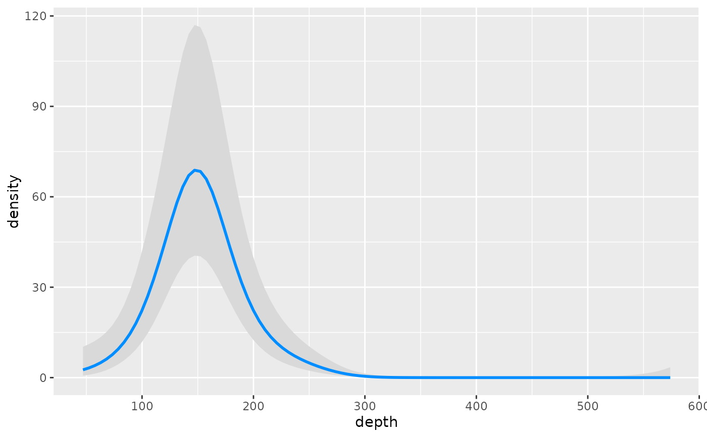
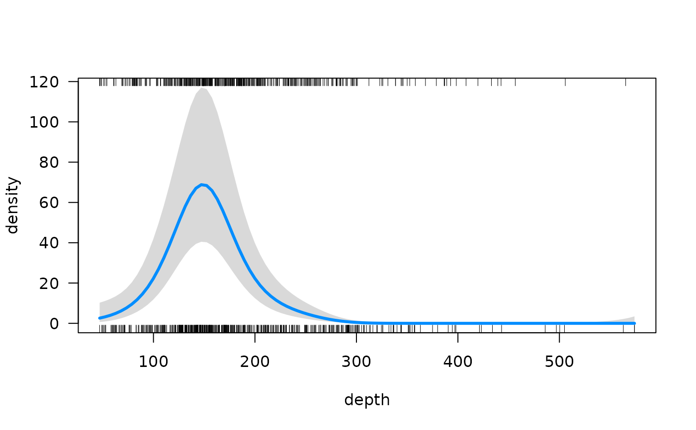 visreg::visreg(fit, xvar = "depth", scale = "response", rug = FALSE)
 # Add spatiotemporal random fields:
fit <- sdmTMB(
density ~ 0 + as.factor(year),
time = "year", #<
data = pcod_2011, mesh = mesh,
family = tweedie(link = "log")
)
fit
#> Spatiotemporal model fit by ML ['sdmTMB']
#> Formula: density ~ 0 + as.factor(year)
#> Mesh: mesh (isotropic covariance)
#> Time column: year
#> Data: pcod_2011
#> Family: tweedie(link = 'log')
#>
#> Conditional model:
#> coef.est coef.se
#> as.factor(year)2011 2.76 0.36
#> as.factor(year)2013 3.10 0.35
#> as.factor(year)2015 3.21 0.35
#> as.factor(year)2017 2.47 0.36
#>
#> Dispersion parameter: 14.83
#> Tweedie p: 1.57
#> Matérn range: 13.31
#> Spatial SD: 3.16
#> Spatiotemporal IID SD: 1.79
#> ML criterion at convergence: 3007.552
#>
#> See ?tidy.sdmTMB to extract these values as a data frame.
# Make the fields AR1:
fit <- sdmTMB(
density ~ s(depth),
time = "year",
spatial = "off",
spatiotemporal = "ar1", #<
data = pcod_2011, mesh = mesh,
family = tweedie(link = "log")
)
fit
#> Spatiotemporal model fit by ML ['sdmTMB']
#> Formula: density ~ s(depth)
#> Mesh: mesh (isotropic covariance)
#> Time column: year
#> Data: pcod_2011
#> Family: tweedie(link = 'log')
#>
#> Conditional model:
#> coef.est coef.se
#> (Intercept) 1.84 0.33
#> sdepth 1.96 3.27
#>
#> Smooth terms:
#> Std. Dev.
#> sd__s(depth) 13.6
#>
#> Dispersion parameter: 12.84
#> Tweedie p: 1.55
#> Spatiotemporal AR1 correlation (rho): 0.67
#> Matérn range: 12.22
#> Spatiotemporal marginal AR1 SD: 3.28
#> ML criterion at convergence: 2914.393
#>
#> See ?tidy.sdmTMB to extract these values as a data frame.
# Make the fields a random walk:
fit <- sdmTMB(
density ~ s(depth),
time = "year",
spatial = "off",
spatiotemporal = "rw", #<
data = pcod_2011, mesh = mesh,
family = tweedie(link = "log")
)
fit
#> Spatiotemporal model fit by ML ['sdmTMB']
#> Formula: density ~ s(depth)
#> Mesh: mesh (isotropic covariance)
#> Time column: year
#> Data: pcod_2011
#> Family: tweedie(link = 'log')
#>
#> Conditional model:
#> coef.est coef.se
#> (Intercept) 1.95 0.34
#> sdepth 1.96 3.18
#>
#> Smooth terms:
#> Std. Dev.
#> sd__s(depth) 13.22
#>
#> Dispersion parameter: 12.84
#> Tweedie p: 1.56
#> Matérn range: 14.66
#> Spatiotemporal RW SD: 2.17
#> ML criterion at convergence: 2919.181
#>
#> See ?tidy.sdmTMB to extract these values as a data frame.
# Depth smoothers by year:
fit <- sdmTMB(
density ~ s(depth, by = as.factor(year)), #<
time = "year",
spatial = "off",
spatiotemporal = "rw",
data = pcod_2011, mesh = mesh,
family = tweedie(link = "log")
)
fit
#> Spatiotemporal model fit by ML ['sdmTMB']
#> Formula: density ~ s(depth, by = as.factor(year))
#> Mesh: mesh (isotropic covariance)
#> Time column: year
#> Data: pcod_2011
#> Family: tweedie(link = 'log')
#>
#> Conditional model:
#> coef.est coef.se
#> (Intercept) 1.76 0.34
#> sdepth):as.factor(year)2011 0.07 4.02
#> sdepth):as.factor(year)2013 4.59 3.28
#> sdepth):as.factor(year)2015 5.97 6.01
#> sdepth):as.factor(year)2017 -1.97 3.22
#>
#> Smooth terms:
#> Std. Dev.
#> sd__s(depth):as.factor(year)2011 16.62
#> sd__s(depth):as.factor(year)2013 13.57
#> sd__s(depth):as.factor(year)2015 28.24
#> sd__s(depth):as.factor(year)2017 18.65
#>
#> Dispersion parameter: 12.70
#> Tweedie p: 1.55
#> Matérn range: 8.62
#> Spatiotemporal RW SD: 3.14
#> ML criterion at convergence: 2924.193
#>
#> See ?tidy.sdmTMB to extract these values as a data frame.
# 2D depth-year smoother:
fit <- sdmTMB(
density ~ s(depth, year), #<
spatial = "off",
data = pcod_2011, mesh = mesh,
family = tweedie(link = "log")
)
fit
#> Model fit by ML ['sdmTMB']
#> Formula: density ~ s(depth, year)
#> Mesh: mesh (isotropic covariance)
#> Data: pcod_2011
#> Family: tweedie(link = 'log')
#>
#> Conditional model:
#> coef.est coef.se
#> (Intercept) 2.55 0.24
#> sdepthyear_1 0.15 0.09
#> sdepthyear_2 2.93 2.07
#>
#> Smooth terms:
#> Std. Dev.
#> sd__s(depth,year) 6.08
#>
#> Dispersion parameter: 14.95
#> Tweedie p: 1.60
#> ML criterion at convergence: 2974.143
#>
#> See ?tidy.sdmTMB to extract these values as a data frame.
# Turn off spatial random fields:
fit <- sdmTMB(
present ~ poly(log(depth)),
spatial = "off", #<
data = pcod_2011, mesh = mesh,
family = binomial()
)
fit
#> Model fit by ML ['sdmTMB']
#> Formula: present ~ poly(log(depth))
#> Mesh: mesh (isotropic covariance)
#> Data: pcod_2011
#> Family: binomial(link = 'logit')
#>
#> Conditional model:
#> coef.est coef.se
#> (Intercept) -0.16 0.07
#> poly(log(depth)) -13.19 2.14
#>
#> ML criterion at convergence: 648.334
#>
#> See ?tidy.sdmTMB to extract these values as a data frame.
# Which matches glm():
fit_glm <- glm(
present ~ poly(log(depth)),
data = pcod_2011,
family = binomial()
)
summary(fit_glm)
#>
#> Call:
#> glm(formula = present ~ poly(log(depth)), family = binomial(),
#> data = pcod_2011)
#>
#> Coefficients:
#> Estimate Std. Error z value Pr(>|z|)
#> (Intercept) -0.16433 0.06583 -2.496 0.0126 *
#> poly(log(depth)) -13.18981 2.14179 -6.158 7.35e-10 ***
#> ---
#> Signif. codes: 0 ‘***’ 0.001 ‘**’ 0.01 ‘*’ 0.05 ‘.’ 0.1 ‘ ’ 1
#>
#> (Dispersion parameter for binomial family taken to be 1)
#>
#> Null deviance: 1337.2 on 968 degrees of freedom
#> Residual deviance: 1296.7 on 967 degrees of freedom
#> AIC: 1300.7
#>
#> Number of Fisher Scoring iterations: 4
#>
AIC(fit, fit_glm)
#> df AIC
#> fit 2 1300.668
#> fit_glm 2 1300.668
# Delta/hurdle binomial-Gamma model:
fit_dg <- sdmTMB(
density ~ poly(log(depth), 2),
data = pcod_2011, mesh = mesh,
spatial = "off",
family = delta_gamma() #<
)
fit_dg
#> Model fit by ML ['sdmTMB']
#> Formula: density ~ poly(log(depth), 2)
#> Mesh: mesh (isotropic covariance)
#> Data: pcod_2011
#> Family: delta_gamma(link1 = 'logit', link2 = 'log')
#>
#> Delta/hurdle model 1: -----------------------------------
#> Family: binomial(link = 'logit')
#> Conditional model:
#> coef.est coef.se
#> (Intercept) -0.48 0.09
#> poly(log(depth), 2)1 -23.06 3.15
#> poly(log(depth), 2)2 -48.79 4.45
#>
#>
#> Delta/hurdle model 2: -----------------------------------
#> Family: Gamma(link = 'log')
#> Conditional model:
#> coef.est coef.se
#> (Intercept) 4.24 0.08
#> poly(log(depth), 2)1 -5.49 3.50
#> poly(log(depth), 2)2 -13.26 3.23
#>
#> Dispersion parameter: 0.64
#>
#> ML criterion at convergence: 2936.579
#>
#> See ?tidy.sdmTMB to extract these values as a data frame.
# Delta model with different formulas and spatial structure:
fit_dg <- sdmTMB(
list(density ~ depth_scaled, density ~ poly(depth_scaled, 2)), #<
data = pcod_2011, mesh = mesh,
spatial = list("off", "on"), #<
family = delta_gamma()
)
fit_dg
#> Spatial model fit by ML ['sdmTMB']
#> Formula: list(density ~ depth_scaled, density ~ poly(depth_scaled, 2))
#> Mesh: mesh (isotropic covariance)
#> Data: pcod_2011
#> Family: delta_gamma(link1 = 'logit', link2 = 'log')
#>
#> Delta/hurdle model 1: -----------------------------------
#> Family: binomial(link = 'logit')
#> Conditional model:
#> coef.est coef.se
#> (Intercept) -0.17 0.07
#> depth_scaled -0.43 0.07
#>
#>
#> Delta/hurdle model 2: -----------------------------------
#> Family: Gamma(link = 'log')
#> Conditional model:
#> coef.est coef.se
#> (Intercept) 4.08 0.14
#> poly(depth_scaled, 2)1 -6.15 4.52
#> poly(depth_scaled, 2)2 -12.58 4.14
#>
#> Dispersion parameter: 0.72
#> Matérn range: 0.01
#> Spatial SD: 2148.71
#>
#> ML criterion at convergence: 3034.512
#>
#> See ?tidy.sdmTMB to extract these values as a data frame.
#>
#> **Possible issues detected! Check output of sanity().**
# Delta/hurdle truncated NB2:
pcod_2011$count <- round(pcod_2011$density)
fit_nb2 <- sdmTMB(
count ~ s(depth),
data = pcod_2011, mesh = mesh,
spatial = "off",
family = delta_truncated_nbinom2() #<
)
fit_nb2
#> Model fit by ML ['sdmTMB']
#> Formula: count ~ s(depth)
#> Mesh: mesh (isotropic covariance)
#> Data: pcod_2011
#> Family: delta_truncated_nbinom2(link1 = 'logit', link2 = 'log')
#>
#> Delta/hurdle model 1: -----------------------------------
#> Family: binomial(link = 'logit')
#> Conditional model:
#> coef.est coef.se
#> (Intercept) -0.69 0.21
#> sdepth 0.29 2.37
#>
#> Smooth terms:
#> Std. Dev.
#> sd__s(depth) 9.6
#>
#>
#> Delta/hurdle model 2: -----------------------------------
#> Family: truncated_nbinom2(link = 'log')
#> Conditional model:
#> coef.est coef.se
#> (Intercept) 4.18 0.22
#> sdepth -0.37 1.77
#>
#> Smooth terms:
#> Std. Dev.
#> sd__s(depth) 6.73
#>
#> Dispersion parameter: 0.49
#>
#> ML criterion at convergence: 2915.733
#>
#> See ?tidy.sdmTMB to extract these values as a data frame.
# Regular NB2:
fit_nb2 <- sdmTMB(
count ~ s(depth),
data = pcod_2011, mesh = mesh,
spatial = "off",
family = nbinom2() #<
)
fit_nb2
#> Model fit by ML ['sdmTMB']
#> Formula: count ~ s(depth)
#> Mesh: mesh (isotropic covariance)
#> Data: pcod_2011
#> Family: nbinom2(link = 'log')
#>
#> Conditional model:
#> coef.est coef.se
#> (Intercept) 2.49 0.27
#> sdepth 3.61 3.96
#>
#> Smooth terms:
#> Std. Dev.
#> sd__s(depth) 16.4
#>
#> Dispersion parameter: 0.14
#> ML criterion at convergence: 3006.939
#>
#> See ?tidy.sdmTMB to extract these values as a data frame.
# IID random intercepts by year:
pcod_2011$fyear <- as.factor(pcod_2011$year)
fit <- sdmTMB(
density ~ s(depth) + (1 | fyear), #<
data = pcod_2011, mesh = mesh,
family = tweedie(link = "log")
)
fit
#> Spatial model fit by ML ['sdmTMB']
#> Formula: density ~ s(depth) + (1 | fyear)
#> Mesh: mesh (isotropic covariance)
#> Data: pcod_2011
#> Family: tweedie(link = 'log')
#>
#> Random intercepts and/or slopes:
#>
#> Conditional model:
#> Groups Name Variance Std.Dev.
#> fyear (Intercept) 0.09 0.30
#>
#> Conditional model:
#> coef.est coef.se
#> (Intercept) 2.13 0.37
#> sdepth 1.82 2.99
#>
#> Smooth terms:
#> Std. Dev.
#> sd__s(depth) 12.51
#>
#> Dispersion parameter: 13.55
#> Tweedie p: 1.58
#> Matérn range: 16.66
#> Spatial SD: 2.21
#> ML criterion at convergence: 2933.138
#>
#> See ?tidy.sdmTMB to extract these values as a data frame.
# Correlated random intercepts and slopes by year:
fit <- sdmTMB(
density ~ (depth | fyear), #<
data = pcod_2011, mesh = mesh,
family = tweedie(link = "log")
)
#> Warning: NaNs produced
#> Warning: The model may not have converged: non-positive-definite Hessian matrix.
# Spatially varying coefficient of year:
pcod_2011$year_scaled <- as.numeric(scale(pcod_2011$year))
fit <- sdmTMB(
density ~ year_scaled,
spatial_varying = ~ 0 + year_scaled, #<
data = pcod_2011, mesh = mesh, family = tweedie(), time = "year"
)
fit
#> Spatiotemporal model fit by ML ['sdmTMB']
#> Formula: density ~ year_scaled
#> Mesh: mesh (isotropic covariance)
#> Time column: year
#> Data: pcod_2011
#> Family: tweedie(link = 'log')
#>
#> Conditional model:
#> coef.est coef.se
#> (Intercept) 2.86 0.33
#> year_scaled -0.06 0.15
#>
#> Dispersion parameter: 14.79
#> Tweedie p: 1.56
#> Matérn range: 20.56
#> Spatial SD: 2.38
#> Spatially varying coefficient SD (year_scaled): 0.81
#> Spatiotemporal IID SD: 1.11
#> ML criterion at convergence: 3008.886
#>
#> See ?tidy.sdmTMB to extract these values as a data frame.
# Time-varying effects of depth and depth squared:
fit <- sdmTMB(
density ~ 0 + as.factor(year),
time_varying = ~ 0 + depth_scaled + depth_scaled2, #<
data = pcod_2011, time = "year", mesh = mesh,
family = tweedie()
)
print(fit)
#> Spatiotemporal model fit by ML ['sdmTMB']
#> Formula: density ~ 0 + as.factor(year)
#> Mesh: mesh (isotropic covariance)
#> Time column: year
#> Data: pcod_2011
#> Family: tweedie(link = 'log')
#>
#> Conditional model:
#> coef.est coef.se
#> as.factor(year)2011 3.73 0.30
#> as.factor(year)2013 3.64 0.28
#> as.factor(year)2015 4.00 0.29
#> as.factor(year)2017 3.31 0.32
#>
#> Time-varying parameters:
#> coef.est coef.se
#> depth_scaled-2011 -1.75 0.32
#> depth_scaled-2013 -1.62 0.26
#> depth_scaled-2015 -1.50 0.27
#> depth_scaled-2017 -2.21 0.46
#> depth_scaled2-2011 -1.92 0.29
#> depth_scaled2-2013 -0.92 0.14
#> depth_scaled2-2015 -1.59 0.22
#> depth_scaled2-2017 -2.20 0.35
#>
#> Dispersion parameter: 12.80
#> Tweedie p: 1.56
#> Matérn range: 0.02
#> Spatial SD: 1512.07
#> Spatiotemporal IID SD: 1227.05
#> ML criterion at convergence: 2910.677
#>
#> See ?tidy.sdmTMB to extract these values as a data frame.
#>
#> **Possible issues detected! Check output of sanity().**
# Extract values:
est <- as.list(fit$sd_report, "Estimate")
se <- as.list(fit$sd_report, "Std. Error")
est$b_rw_t[, , 1]
#> [,1] [,2]
#> [1,] -1.747608 -1.9199717
#> [2,] -1.623032 -0.9195933
#> [3,] -1.502954 -1.5858305
#> [4,] -2.212812 -2.1992567
se$b_rw_t[, , 1]
#> [,1] [,2]
#> [1,] 0.3239487 0.2944086
#> [2,] 0.2574118 0.1386946
#> [3,] 0.2692363 0.2197914
#> [4,] 0.4611855 0.3514651
# Linear break-point effect of depth:
fit <- sdmTMB(
density ~ breakpt(depth_scaled), #<
data = pcod_2011,
mesh = mesh,
family = tweedie()
)
#> Warning: The model may not have converged. Maximum final gradient: 1.72126009333005.
fit
#> Spatial model fit by ML ['sdmTMB']
#> Formula: density ~ breakpt(depth_scaled)
#> Mesh: mesh (isotropic covariance)
#> Data: pcod_2011
#> Family: tweedie(link = 'log')
#>
#> Conditional model:
#> coef.est coef.se
#> (Intercept) 5.00 0.62
#> depth_scaled-slope 2.04 0.39
#> depth_scaled-breakpt -0.87 0.02
#>
#> Dispersion parameter: 15.22
#> Tweedie p: 1.59
#> Matérn range: 41.74
#> Spatial SD: 1.96
#> ML criterion at convergence: 3008.808
#>
#> See ?tidy.sdmTMB to extract these values as a data frame.
#>
#> **Possible issues detected! Check output of sanity().**
# }
# Add spatiotemporal random fields:
fit <- sdmTMB(
density ~ 0 + as.factor(year),
time = "year", #<
data = pcod_2011, mesh = mesh,
family = tweedie(link = "log")
)
fit
#> Spatiotemporal model fit by ML ['sdmTMB']
#> Formula: density ~ 0 + as.factor(year)
#> Mesh: mesh (isotropic covariance)
#> Time column: year
#> Data: pcod_2011
#> Family: tweedie(link = 'log')
#>
#> Conditional model:
#> coef.est coef.se
#> as.factor(year)2011 2.76 0.36
#> as.factor(year)2013 3.10 0.35
#> as.factor(year)2015 3.21 0.35
#> as.factor(year)2017 2.47 0.36
#>
#> Dispersion parameter: 14.83
#> Tweedie p: 1.57
#> Matérn range: 13.31
#> Spatial SD: 3.16
#> Spatiotemporal IID SD: 1.79
#> ML criterion at convergence: 3007.552
#>
#> See ?tidy.sdmTMB to extract these values as a data frame.
# Make the fields AR1:
fit <- sdmTMB(
density ~ s(depth),
time = "year",
spatial = "off",
spatiotemporal = "ar1", #<
data = pcod_2011, mesh = mesh,
family = tweedie(link = "log")
)
fit
#> Spatiotemporal model fit by ML ['sdmTMB']
#> Formula: density ~ s(depth)
#> Mesh: mesh (isotropic covariance)
#> Time column: year
#> Data: pcod_2011
#> Family: tweedie(link = 'log')
#>
#> Conditional model:
#> coef.est coef.se
#> (Intercept) 1.84 0.33
#> sdepth 1.96 3.27
#>
#> Smooth terms:
#> Std. Dev.
#> sd__s(depth) 13.6
#>
#> Dispersion parameter: 12.84
#> Tweedie p: 1.55
#> Spatiotemporal AR1 correlation (rho): 0.67
#> Matérn range: 12.22
#> Spatiotemporal marginal AR1 SD: 3.28
#> ML criterion at convergence: 2914.393
#>
#> See ?tidy.sdmTMB to extract these values as a data frame.
# Make the fields a random walk:
fit <- sdmTMB(
density ~ s(depth),
time = "year",
spatial = "off",
spatiotemporal = "rw", #<
data = pcod_2011, mesh = mesh,
family = tweedie(link = "log")
)
fit
#> Spatiotemporal model fit by ML ['sdmTMB']
#> Formula: density ~ s(depth)
#> Mesh: mesh (isotropic covariance)
#> Time column: year
#> Data: pcod_2011
#> Family: tweedie(link = 'log')
#>
#> Conditional model:
#> coef.est coef.se
#> (Intercept) 1.95 0.34
#> sdepth 1.96 3.18
#>
#> Smooth terms:
#> Std. Dev.
#> sd__s(depth) 13.22
#>
#> Dispersion parameter: 12.84
#> Tweedie p: 1.56
#> Matérn range: 14.66
#> Spatiotemporal RW SD: 2.17
#> ML criterion at convergence: 2919.181
#>
#> See ?tidy.sdmTMB to extract these values as a data frame.
# Depth smoothers by year:
fit <- sdmTMB(
density ~ s(depth, by = as.factor(year)), #<
time = "year",
spatial = "off",
spatiotemporal = "rw",
data = pcod_2011, mesh = mesh,
family = tweedie(link = "log")
)
fit
#> Spatiotemporal model fit by ML ['sdmTMB']
#> Formula: density ~ s(depth, by = as.factor(year))
#> Mesh: mesh (isotropic covariance)
#> Time column: year
#> Data: pcod_2011
#> Family: tweedie(link = 'log')
#>
#> Conditional model:
#> coef.est coef.se
#> (Intercept) 1.76 0.34
#> sdepth):as.factor(year)2011 0.07 4.02
#> sdepth):as.factor(year)2013 4.59 3.28
#> sdepth):as.factor(year)2015 5.97 6.01
#> sdepth):as.factor(year)2017 -1.97 3.22
#>
#> Smooth terms:
#> Std. Dev.
#> sd__s(depth):as.factor(year)2011 16.62
#> sd__s(depth):as.factor(year)2013 13.57
#> sd__s(depth):as.factor(year)2015 28.24
#> sd__s(depth):as.factor(year)2017 18.65
#>
#> Dispersion parameter: 12.70
#> Tweedie p: 1.55
#> Matérn range: 8.62
#> Spatiotemporal RW SD: 3.14
#> ML criterion at convergence: 2924.193
#>
#> See ?tidy.sdmTMB to extract these values as a data frame.
# 2D depth-year smoother:
fit <- sdmTMB(
density ~ s(depth, year), #<
spatial = "off",
data = pcod_2011, mesh = mesh,
family = tweedie(link = "log")
)
fit
#> Model fit by ML ['sdmTMB']
#> Formula: density ~ s(depth, year)
#> Mesh: mesh (isotropic covariance)
#> Data: pcod_2011
#> Family: tweedie(link = 'log')
#>
#> Conditional model:
#> coef.est coef.se
#> (Intercept) 2.55 0.24
#> sdepthyear_1 0.15 0.09
#> sdepthyear_2 2.93 2.07
#>
#> Smooth terms:
#> Std. Dev.
#> sd__s(depth,year) 6.08
#>
#> Dispersion parameter: 14.95
#> Tweedie p: 1.60
#> ML criterion at convergence: 2974.143
#>
#> See ?tidy.sdmTMB to extract these values as a data frame.
# Turn off spatial random fields:
fit <- sdmTMB(
present ~ poly(log(depth)),
spatial = "off", #<
data = pcod_2011, mesh = mesh,
family = binomial()
)
fit
#> Model fit by ML ['sdmTMB']
#> Formula: present ~ poly(log(depth))
#> Mesh: mesh (isotropic covariance)
#> Data: pcod_2011
#> Family: binomial(link = 'logit')
#>
#> Conditional model:
#> coef.est coef.se
#> (Intercept) -0.16 0.07
#> poly(log(depth)) -13.19 2.14
#>
#> ML criterion at convergence: 648.334
#>
#> See ?tidy.sdmTMB to extract these values as a data frame.
# Which matches glm():
fit_glm <- glm(
present ~ poly(log(depth)),
data = pcod_2011,
family = binomial()
)
summary(fit_glm)
#>
#> Call:
#> glm(formula = present ~ poly(log(depth)), family = binomial(),
#> data = pcod_2011)
#>
#> Coefficients:
#> Estimate Std. Error z value Pr(>|z|)
#> (Intercept) -0.16433 0.06583 -2.496 0.0126 *
#> poly(log(depth)) -13.18981 2.14179 -6.158 7.35e-10 ***
#> ---
#> Signif. codes: 0 ‘***’ 0.001 ‘**’ 0.01 ‘*’ 0.05 ‘.’ 0.1 ‘ ’ 1
#>
#> (Dispersion parameter for binomial family taken to be 1)
#>
#> Null deviance: 1337.2 on 968 degrees of freedom
#> Residual deviance: 1296.7 on 967 degrees of freedom
#> AIC: 1300.7
#>
#> Number of Fisher Scoring iterations: 4
#>
AIC(fit, fit_glm)
#> df AIC
#> fit 2 1300.668
#> fit_glm 2 1300.668
# Delta/hurdle binomial-Gamma model:
fit_dg <- sdmTMB(
density ~ poly(log(depth), 2),
data = pcod_2011, mesh = mesh,
spatial = "off",
family = delta_gamma() #<
)
fit_dg
#> Model fit by ML ['sdmTMB']
#> Formula: density ~ poly(log(depth), 2)
#> Mesh: mesh (isotropic covariance)
#> Data: pcod_2011
#> Family: delta_gamma(link1 = 'logit', link2 = 'log')
#>
#> Delta/hurdle model 1: -----------------------------------
#> Family: binomial(link = 'logit')
#> Conditional model:
#> coef.est coef.se
#> (Intercept) -0.48 0.09
#> poly(log(depth), 2)1 -23.06 3.15
#> poly(log(depth), 2)2 -48.79 4.45
#>
#>
#> Delta/hurdle model 2: -----------------------------------
#> Family: Gamma(link = 'log')
#> Conditional model:
#> coef.est coef.se
#> (Intercept) 4.24 0.08
#> poly(log(depth), 2)1 -5.49 3.50
#> poly(log(depth), 2)2 -13.26 3.23
#>
#> Dispersion parameter: 0.64
#>
#> ML criterion at convergence: 2936.579
#>
#> See ?tidy.sdmTMB to extract these values as a data frame.
# Delta model with different formulas and spatial structure:
fit_dg <- sdmTMB(
list(density ~ depth_scaled, density ~ poly(depth_scaled, 2)), #<
data = pcod_2011, mesh = mesh,
spatial = list("off", "on"), #<
family = delta_gamma()
)
fit_dg
#> Spatial model fit by ML ['sdmTMB']
#> Formula: list(density ~ depth_scaled, density ~ poly(depth_scaled, 2))
#> Mesh: mesh (isotropic covariance)
#> Data: pcod_2011
#> Family: delta_gamma(link1 = 'logit', link2 = 'log')
#>
#> Delta/hurdle model 1: -----------------------------------
#> Family: binomial(link = 'logit')
#> Conditional model:
#> coef.est coef.se
#> (Intercept) -0.17 0.07
#> depth_scaled -0.43 0.07
#>
#>
#> Delta/hurdle model 2: -----------------------------------
#> Family: Gamma(link = 'log')
#> Conditional model:
#> coef.est coef.se
#> (Intercept) 4.08 0.14
#> poly(depth_scaled, 2)1 -6.15 4.52
#> poly(depth_scaled, 2)2 -12.58 4.14
#>
#> Dispersion parameter: 0.72
#> Matérn range: 0.01
#> Spatial SD: 2148.71
#>
#> ML criterion at convergence: 3034.512
#>
#> See ?tidy.sdmTMB to extract these values as a data frame.
#>
#> **Possible issues detected! Check output of sanity().**
# Delta/hurdle truncated NB2:
pcod_2011$count <- round(pcod_2011$density)
fit_nb2 <- sdmTMB(
count ~ s(depth),
data = pcod_2011, mesh = mesh,
spatial = "off",
family = delta_truncated_nbinom2() #<
)
fit_nb2
#> Model fit by ML ['sdmTMB']
#> Formula: count ~ s(depth)
#> Mesh: mesh (isotropic covariance)
#> Data: pcod_2011
#> Family: delta_truncated_nbinom2(link1 = 'logit', link2 = 'log')
#>
#> Delta/hurdle model 1: -----------------------------------
#> Family: binomial(link = 'logit')
#> Conditional model:
#> coef.est coef.se
#> (Intercept) -0.69 0.21
#> sdepth 0.29 2.37
#>
#> Smooth terms:
#> Std. Dev.
#> sd__s(depth) 9.6
#>
#>
#> Delta/hurdle model 2: -----------------------------------
#> Family: truncated_nbinom2(link = 'log')
#> Conditional model:
#> coef.est coef.se
#> (Intercept) 4.18 0.22
#> sdepth -0.37 1.77
#>
#> Smooth terms:
#> Std. Dev.
#> sd__s(depth) 6.73
#>
#> Dispersion parameter: 0.49
#>
#> ML criterion at convergence: 2915.733
#>
#> See ?tidy.sdmTMB to extract these values as a data frame.
# Regular NB2:
fit_nb2 <- sdmTMB(
count ~ s(depth),
data = pcod_2011, mesh = mesh,
spatial = "off",
family = nbinom2() #<
)
fit_nb2
#> Model fit by ML ['sdmTMB']
#> Formula: count ~ s(depth)
#> Mesh: mesh (isotropic covariance)
#> Data: pcod_2011
#> Family: nbinom2(link = 'log')
#>
#> Conditional model:
#> coef.est coef.se
#> (Intercept) 2.49 0.27
#> sdepth 3.61 3.96
#>
#> Smooth terms:
#> Std. Dev.
#> sd__s(depth) 16.4
#>
#> Dispersion parameter: 0.14
#> ML criterion at convergence: 3006.939
#>
#> See ?tidy.sdmTMB to extract these values as a data frame.
# IID random intercepts by year:
pcod_2011$fyear <- as.factor(pcod_2011$year)
fit <- sdmTMB(
density ~ s(depth) + (1 | fyear), #<
data = pcod_2011, mesh = mesh,
family = tweedie(link = "log")
)
fit
#> Spatial model fit by ML ['sdmTMB']
#> Formula: density ~ s(depth) + (1 | fyear)
#> Mesh: mesh (isotropic covariance)
#> Data: pcod_2011
#> Family: tweedie(link = 'log')
#>
#> Random intercepts and/or slopes:
#>
#> Conditional model:
#> Groups Name Variance Std.Dev.
#> fyear (Intercept) 0.09 0.30
#>
#> Conditional model:
#> coef.est coef.se
#> (Intercept) 2.13 0.37
#> sdepth 1.82 2.99
#>
#> Smooth terms:
#> Std. Dev.
#> sd__s(depth) 12.51
#>
#> Dispersion parameter: 13.55
#> Tweedie p: 1.58
#> Matérn range: 16.66
#> Spatial SD: 2.21
#> ML criterion at convergence: 2933.138
#>
#> See ?tidy.sdmTMB to extract these values as a data frame.
# Correlated random intercepts and slopes by year:
fit <- sdmTMB(
density ~ (depth | fyear), #<
data = pcod_2011, mesh = mesh,
family = tweedie(link = "log")
)
#> Warning: NaNs produced
#> Warning: The model may not have converged: non-positive-definite Hessian matrix.
# Spatially varying coefficient of year:
pcod_2011$year_scaled <- as.numeric(scale(pcod_2011$year))
fit <- sdmTMB(
density ~ year_scaled,
spatial_varying = ~ 0 + year_scaled, #<
data = pcod_2011, mesh = mesh, family = tweedie(), time = "year"
)
fit
#> Spatiotemporal model fit by ML ['sdmTMB']
#> Formula: density ~ year_scaled
#> Mesh: mesh (isotropic covariance)
#> Time column: year
#> Data: pcod_2011
#> Family: tweedie(link = 'log')
#>
#> Conditional model:
#> coef.est coef.se
#> (Intercept) 2.86 0.33
#> year_scaled -0.06 0.15
#>
#> Dispersion parameter: 14.79
#> Tweedie p: 1.56
#> Matérn range: 20.56
#> Spatial SD: 2.38
#> Spatially varying coefficient SD (year_scaled): 0.81
#> Spatiotemporal IID SD: 1.11
#> ML criterion at convergence: 3008.886
#>
#> See ?tidy.sdmTMB to extract these values as a data frame.
# Time-varying effects of depth and depth squared:
fit <- sdmTMB(
density ~ 0 + as.factor(year),
time_varying = ~ 0 + depth_scaled + depth_scaled2, #<
data = pcod_2011, time = "year", mesh = mesh,
family = tweedie()
)
print(fit)
#> Spatiotemporal model fit by ML ['sdmTMB']
#> Formula: density ~ 0 + as.factor(year)
#> Mesh: mesh (isotropic covariance)
#> Time column: year
#> Data: pcod_2011
#> Family: tweedie(link = 'log')
#>
#> Conditional model:
#> coef.est coef.se
#> as.factor(year)2011 3.73 0.30
#> as.factor(year)2013 3.64 0.28
#> as.factor(year)2015 4.00 0.29
#> as.factor(year)2017 3.31 0.32
#>
#> Time-varying parameters:
#> coef.est coef.se
#> depth_scaled-2011 -1.75 0.32
#> depth_scaled-2013 -1.62 0.26
#> depth_scaled-2015 -1.50 0.27
#> depth_scaled-2017 -2.21 0.46
#> depth_scaled2-2011 -1.92 0.29
#> depth_scaled2-2013 -0.92 0.14
#> depth_scaled2-2015 -1.59 0.22
#> depth_scaled2-2017 -2.20 0.35
#>
#> Dispersion parameter: 12.80
#> Tweedie p: 1.56
#> Matérn range: 0.02
#> Spatial SD: 1512.07
#> Spatiotemporal IID SD: 1227.05
#> ML criterion at convergence: 2910.677
#>
#> See ?tidy.sdmTMB to extract these values as a data frame.
#>
#> **Possible issues detected! Check output of sanity().**
# Extract values:
est <- as.list(fit$sd_report, "Estimate")
se <- as.list(fit$sd_report, "Std. Error")
est$b_rw_t[, , 1]
#> [,1] [,2]
#> [1,] -1.747608 -1.9199717
#> [2,] -1.623032 -0.9195933
#> [3,] -1.502954 -1.5858305
#> [4,] -2.212812 -2.1992567
se$b_rw_t[, , 1]
#> [,1] [,2]
#> [1,] 0.3239487 0.2944086
#> [2,] 0.2574118 0.1386946
#> [3,] 0.2692363 0.2197914
#> [4,] 0.4611855 0.3514651
# Linear break-point effect of depth:
fit <- sdmTMB(
density ~ breakpt(depth_scaled), #<
data = pcod_2011,
mesh = mesh,
family = tweedie()
)
#> Warning: The model may not have converged. Maximum final gradient: 1.72126009333005.
fit
#> Spatial model fit by ML ['sdmTMB']
#> Formula: density ~ breakpt(depth_scaled)
#> Mesh: mesh (isotropic covariance)
#> Data: pcod_2011
#> Family: tweedie(link = 'log')
#>
#> Conditional model:
#> coef.est coef.se
#> (Intercept) 5.00 0.62
#> depth_scaled-slope 2.04 0.39
#> depth_scaled-breakpt -0.87 0.02
#>
#> Dispersion parameter: 15.22
#> Tweedie p: 1.59
#> Matérn range: 41.74
#> Spatial SD: 1.96
#> ML criterion at convergence: 3008.808
#>
#> See ?tidy.sdmTMB to extract these values as a data frame.
#>
#> **Possible issues detected! Check output of sanity().**
# }