Prior distributions

Optional priors/penalties on model parameters. This results in penalized likelihood within TMB or can be used as priors if the model is passed to tmbstan (see the Bayesian vignette).

Note that Jacobian adjustments are only made if bayesian = TRUE when the sdmTMB() model is fit. In other words, if the final model will be fit with tmbstan and priors are specified, then bayesian should be set to TRUE. Otherwise, leave bayesian = FALSE.

pc_matern() is the Penalized Complexity prior for the Matérn covariance function.

Usage

sdmTMBpriors(
  matern_s = pc_matern(range_gt = NA, sigma_lt = NA),
  matern_st = pc_matern(range_gt = NA, sigma_lt = NA),
  phi = halfnormal(NA, NA),
  ar1_rho = normal(NA, NA),
  tweedie_p = normal(NA, NA),
  b = normal(NA, NA),
  sigma_V = gamma_cv(NA, NA),
  threshold_breakpt_slope = normal(NA, NA),
  threshold_breakpt_cut = normal(NA, NA),
  threshold_logistic_s50 = normal(NA, NA),
  threshold_logistic_s95 = normal(NA, NA),
  threshold_logistic_smax = normal(NA, NA),
  custom = NULL,
  custom_log_jacobian = NULL
)

normal(location = 0, scale = 1)

halfnormal(location = 0, scale = 1)

gamma_cv(location, cv)

lognormal_prior(meanlog, sdlog)

mvnormal(location = 0, scale = diag(length(location)))

pc_matern(range_gt, sigma_lt, range_prob = 0.05, sigma_prob = 0.05)

Arguments

matern_s: A PC (Penalized Complexity) prior (pc_matern()) on the spatial random field Matérn parameters.
matern_st: Same as matern_s but for the spatiotemporal random field. Note that you will likely want to set share_range = FALSE if you choose to set both a spatial and spatiotemporal Matérn PC prior since they both include a prior on the spatial range parameter.
phi: A halfnormal() prior for the dispersion parameter in the observation distribution.
ar1_rho: A normal() prior for the AR1 random field parameter. Note the parameter has support -1 < ar1_rho < 1.
tweedie_p: A normal() prior for the Tweedie power parameter. Note the parameter has support 1 < tweedie_p < 2 so choose a mean appropriately.
b: normal() priors for the main population-level 'beta' effects.
sigma_V: gamma_cv() or lognormal_prior() priors for any time-varying parameter SDs. Supply a single prior to apply it to all time-varying coefficients or a vector with one element per coefficient (NA for no prior). In delta models, the priors apply to both components.
threshold_breakpt_slope: A normal() prior for the slope of the linear (hockey stick) function.
threshold_breakpt_cut: A normal() prior for the cutoff of the linear (hockey stick) function.
threshold_logistic_s50: A normal() prior for the parameter at which f(x) = 0.5.
threshold_logistic_s95: A normal() prior for the parameter at which f(x) = 0.95.
threshold_logistic_smax: A normal() prior for the parameter at which f(x) is maximized.
custom: Optional function of (par, theta) returning one or more log density contributions (RTMB backend only; see Custom priors below).
custom_log_jacobian: Optional function of (par, theta) returning the log absolute Jacobian for custom. Only used if bayesian = TRUE. Requires custom.
location: Location parameter(s). Typically the mean.
scale: Scale parameter. For normal()/halfnormal(): standard deviation(s). For mvnormal(): variance-covariance matrix.
cv: Coefficient of variation (SD/mean).
meanlog: Mean of the distribution on the log scale.
sdlog: Standard deviation of the distribution on the log scale.
range_gt: A value one expects the spatial or spatiotemporal range is greater than with 1 - range_prob probability.
sigma_lt: A value one expects the spatial or spatiotemporal marginal standard deviation (sigma_O or sigma_E internally) is less than with 1 - sigma_prob probability.
range_prob: Probability. See description for range_gt.
sigma_prob: Probability. See description for sigma_lt.

Value

A named list with values for the specified priors.

Details

Pass these objects to the priors argument in sdmTMB().

normal() and halfnormal() define normal and half-normal priors that, for now, must have a location (mean) parameter of 0. halfnormal() is the same as normal() but can be used to make the syntax clearer. It is intended to be used for parameters that have support > 0.

See https://arxiv.org/abs/1503.00256 for a description of the PC prior for Gaussian random fields. Quoting the discussion (and substituting the argument names in pc_matern()): "In the simulation study we observe good coverage of the equal-tailed 95% credible intervals when the prior satisfies P(sigma > sigma_lt) = 0.05 and P(range < range_gt) = 0.05, where sigma_lt is between 2.5 to 40 times the true marginal standard deviation and range_gt is between 1/10 and 1/2.5 of the true range."

Keep in mind that the range is dependent on the units and scale of the coordinate system. In practice, you may choose to try fitting the model without a PC prior and then constraining the model from there. A better option would be to simulate from a model with a given range and sigma to choose reasonable values for the system or base the prior on knowledge from a model fit to a similar system but with more spatial information in the data.

lognormal_prior() defines a lognormal prior with the same parameterization as stats::dlnorm(). The median is exp(meanlog).

Custom priors

With the RTMB backend (the default), custom adds arbitrary log densities to the joint objective. The function is called as custom(par, theta), where par is the list of raw (internal) parameters and theta is a list of natural-scale versions of them. See get_prior_parameters() for their names, shapes, and labels. It must return a numeric scalar, vector, or array of log densities (names are optional), which are summed and subtracted from the negative log likelihood. Custom terms are evaluated inside the objective, so they are included in gradients, Hessians, the Laplace approximation, and standard errors, and may involve random effects. They supplement, rather than replace, the built-in priors and random effect distributions. Use get_prior_densities() to see the contributions at the estimated parameters.

The function must:

use operations and densities that RTMB can differentiate, such as RTMB::dnorm(x, mean, sd, log = TRUE); stats::dnorm() can't take AD values;
return log densities (remember log = TRUE, which can't be checked);
not branch on parameter values (e.g., if (par$b_j[1] > 0));
be deterministic and free of side effects;
also work on ordinary numeric inputs.

Fixed hyperparameters can be defined in the function's enclosing environment. The functions are saved with the fitted model, so keep their environments small (e.g., avoid defining them inside a function holding large data).

Jacobians. With bayesian = FALSE, custom priors are penalties: the optimum is the posterior mode on the scale the prior is written on, and no Jacobian is needed. With bayesian = TRUE (e.g., for sampling with tmbstan), the result of custom_log_jacobian(par, theta) is also added. No Jacobian adjustment is ever inferred: without custom_log_jacobian, a prior on a transformed parameter (e.g., theta$phi) is not a valid prior density on that parameter's natural scale for sampling. For a prior on phi = exp(ln_phi), the log Jacobian is par$ln_phi.

Matérn range and SDs. The Matérn range and the field SDs (sigma_O, sigma_E) are more complex than most parameters because they depend on each other: each SD is a function of both ln_tau_* and ln_kappa. A Jacobian for one of them alone isn't well defined; it needs the joint transformation from (ln_kappa, ln_tau_*) to (range, sigma_*), whose log Jacobian is log(range) + log(sigma_*). With a shared range (the default), add log(range) once plus log(sigma_*) for each field. For priors on these parameters we suggest the built-in PC priors, pc_matern() via the matern_s and matern_st arguments, which apply the Jacobian for you if bayesian = TRUE.

Limitations. Custom terms are not evaluated in the first phase of sdmTMBcontrol(multiphase = TRUE), which only finds starting values with random fields turned off. Custom priors do not define a sampler: simulate.sdmTMB() and other simulation methods ignore any change that custom terms make to the distribution of random effects. Held-out log likelihoods in sdmTMB_cv() exclude all priors. As with the built-in priors, custom terms are part of the objective, so they are included in stats::logLik() and stats::AIC().

References

Fuglstad, G.-A., Simpson, D., Lindgren, F., and Rue, H. (2016) Constructing Priors that Penalize the Complexity of Gaussian Random Fields. arXiv:1503.00256

Simpson, D., Rue, H., Martins, T., Riebler, A., and Sørbye, S. (2015) Penalising model component complexity: A principled, practical approach to constructing priors. arXiv:1403.4630

Examples

normal(0, 1)
#>      [,1] [,2]
#> [1,]    0    1
#> attr(,"dist")
#> [1] "normal"
halfnormal(0, 1)
#>      [,1] [,2]
#> [1,]    0    1
#> attr(,"dist")
#> [1] "normal"
gamma_cv(0.5, 0.2)
#>      [,1] [,2]
#> [1,]   25 0.02
#> attr(,"dist")
#> [1] "gamma"
lognormal_prior(log(0.2), 0.5)
#>           [,1] [,2]
#> [1,] -1.609438  0.5
#> attr(,"dist")
#> [1] "lognormal"
mvnormal(c(0, 0))
#>      [,1] [,2] [,3]
#> [1,]    0    1    0
#> [2,]    0    0    1
#> attr(,"dist")
#> [1] "mvnormal"
pc_matern(range_gt = 5, sigma_lt = 1)
#> [1] 5.00 1.00 0.05 0.05
#> attr(,"dist")
#> [1] "pc_matern"
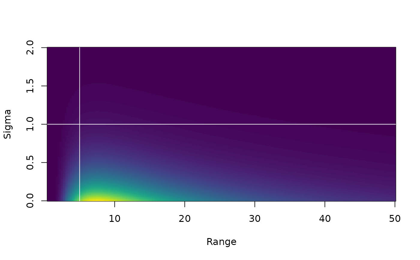
plot_pc_matern(range_gt = 5, sigma_lt = 1)


# \donttest{
d <- subset(pcod, year > 2011)
pcod_spde <- make_mesh(d, c("X", "Y"), cutoff = 30)

# - no priors on population-level effects (`b`)
# - halfnormal(0, 10) prior on dispersion parameter `phi`
# - Matern PC priors on spatial `matern_s` and spatiotemporal
#   `matern_st` random field parameters
m <- sdmTMB(density ~ s(depth, k = 3),
  data = d, mesh = pcod_spde, family = tweedie(),
  share_range = FALSE, time = "year",
  priors = sdmTMBpriors(
    phi = halfnormal(0, 10),
    matern_s = pc_matern(range_gt = 5, sigma_lt = 1),
    matern_st = pc_matern(range_gt = 5, sigma_lt = 1)
  )
)

# - no prior on intercept
# - normal(0, 1) prior on depth coefficient
# - no prior on the dispersion parameter `phi`
# - Matern PC prior
m <- sdmTMB(density ~ depth_scaled,
  data = d, mesh = pcod_spde, family = tweedie(),
  spatiotemporal = "off",
  priors = sdmTMBpriors(
    b = normal(c(NA, 0), c(NA, 1)),
    matern_s = pc_matern(range_gt = 5, sigma_lt = 1)
  )
)

# You get a prior, you get a prior, you get a prior!
# (except on the annual means; see the `NA`s)
m <- sdmTMB(density ~ 0 + depth_scaled + depth_scaled2 + as.factor(year),
  data = d, time = "year", mesh = pcod_spde, family = tweedie(link = "log"),
  share_range = FALSE, spatiotemporal = "AR1",
  priors = sdmTMBpriors(
    b = normal(c(0, 0, NA, NA, NA), c(2, 2, NA, NA, NA)),
    phi = halfnormal(0, 10),
    # tweedie_p = normal(1.5, 2),
    ar1_rho = normal(0, 1),
    matern_s = pc_matern(range_gt = 5, sigma_lt = 1),
    matern_st = pc_matern(range_gt = 5, sigma_lt = 1))
)
# }