Make predictions from an sdmTMB model. Predictions can be made on the original data or on new data.
Usage
# S3 method for class 'sdmTMB'
predict(
  object,
  newdata = NULL,
  type = c("link", "response"),
  se_fit = FALSE,
  re_form = NULL,
  re_form_iid = NULL,
  allow_new_levels = NULL,
  nsim = 0,
  sims_var = "est",
  model = c(NA, 1, 2),
  offset = NULL,
  mcmc_samples = NULL,
  nonlocal_newdata = NULL,
  return_tmb_object = FALSE,
  return_tmb_report = FALSE,
  return_tmb_data = FALSE,
  ...
)
Arguments
- object
A model fitted with
sdmTMB().- newdata
A data frame to make predictions on. It should contain the same predictor columns as the fitted data and, for spatiotemporal models, a time column with the same name as in the fitted data.
- type
Should predictions be returned in link space (default) or response space?
- se_fit
Should standard errors on predictions be calculated? Warning: can be slow for large datasets or high-resolution projections when random fields are included. For faster uncertainty estimation, either use
re_form = NAto exclude random fields or use thensimargument to simulate from the joint precision matrix.- re_form
NULLto include all spatial/spatiotemporal random fields in predictions.~0orNAfor population-level predictions (predictions excluding spatial/spatiotemporal random fields). Often used withse_fit = TRUEto visualize marginal effects. Does not affectget_index()calculations.- re_form_iid
NULLto include all IID random intercepts/slopes in the predictions.~0orNAfor population-level predictions. No other options (e.g., some but not all random intercepts) are not yet implemented. Only affects predictions withnewdata. This does affectget_index().- allow_new_levels
Logical or
NULL. Similar to glmmTMB'sallow.new.levels. Allows predictions for previously unobserved levels in random effect grouping variables. IfNULL(default), new levels are allowed whenre_form_iid = NAorre_form_iid = ~0and a warning is issued otherwise. IfTRUE, new levels are explicitly allowed. IfFALSE, a warning is issued if new levels are found. New levels are always treated as population-level predictions for the IID random effects (i.e., random effect value = 0).- nsim
If
> 0, simulate from the joint precision matrix withnsimdraws. Returns a matrix with one row per prediction location and one column per draw. By default, each column represents one draw of the linear predictor in link space; usetype = "response"for response-space draws. Simulating from the joint precision matrix accounts for uncertainty in both fixed and random effects. Use this to derive uncertainty on predictions (e.g.,apply(x, 1, sd)) or propagate uncertainty to derived quantities. This is the fastest way to characterize spatial uncertainty with sdmTMB.- sims_var
Experimental: Which TMB reported variable from the model should be extracted from the joint precision matrix simulation draws? Defaults to link-space predictions. Options include:
"omega_s","zeta_s","epsilon_st", and"est_rf"(as described below). Other options will be passed verbatim.- model
Which component to predict from delta/hurdle models when
nsim > 0ormcmc_samplesis supplied.NA(default) returns the combined prediction from both components;1returns the binomial component only;2returns the positive component only. Predictions are on the link or response scale depending ontype. For regular predictions (without simulation), both components are returned. See the delta-model vignette.- offset
A numeric vector of optional offset values. When predictions are made with
newdataor with options that internally rebuild prediction data (e.g.,type = "response",se_fit = TRUE, ornsim > 0), the defaultNULLuses an offset of 0. The simplestpredict(object)call on the original data uses the offset from the fitted model.- mcmc_samples
See
extract_mcmc()in the sdmTMBextra package for more details and the Bayesian vignette. If specified, the predict function will return a matrix of a similar form as ifnsim > 0but representing Bayesian posterior samples from the Stan model.- nonlocal_newdata
An optional data frame overriding the
nonlocal_formulacovariate field used for prediction (e.g., for a counterfactual/scenario surface), with the same requirements asnonlocal_datainsdmTMB().newdata's x/y and time columns always determine where predictions are projected to; this argument only controls where the underlying diffused covariate values come from. Defaults toNULL: if a grid was supplied at fit time, the fitted field is reused as-is (sonewdataneed not contain the diffusion covariate columns); otherwise the field is rebuilt fromnewdata's own covariate columns, as before.- return_tmb_object
Logical. If
TRUE, include the TMB object in a list-format output. Necessary for theget_index()orget_cog()functions.- return_tmb_report
Logical: return the output from the TMB report? For regular prediction, this is all the reported variables at the MLE parameter values. For
nsim > 0or whenmcmc_samplesis supplied, this is a list with one element per sample; each element contains the report output for that sample.- return_tmb_data
Logical: return formatted data for TMB? Used internally.
- ...
Unused.
Value
If return_tmb_object = FALSE (and nsim = 0 and mcmc_samples = NULL):
A data frame:
est: Estimate in link or response space, depending ontypeest_non_rf: Estimate from everything except spatial/spatiotemporal random fields (fixed effects, random intercepts, time-varying effects, etc.)est_rf: Estimate from all random fields combinedomega_s: Spatial random field (models consistent spatial patterns)zeta_s: Spatially varying coefficient field (models how effects vary across space)epsilon_st: Spatiotemporal random field (models spatial patterns that vary over time)nl_*: Nonlocal transformed covariate values (one column per nonlocal term; available whennonlocal_formulaterms were fitted)
Delta/hurdle models return component-specific columns with 1 and 2
suffixes for the binomial and positive components, respectively (e.g.,
est1, est2, omega_s1, omega_s2). With type = "response",
est is the combined response-scale prediction.
If return_tmb_object = TRUE (and nsim = 0 and mcmc_samples = NULL):
A list:
data: The data frame described abovereport: The TMB report on parameter valuesobj: The TMB object returned from the prediction runfit_obj: The original TMB model object
In this case, you likely only need the data element as an end user.
The other elements are included for other functions.
If nsim > 0 or mcmc_samples is not NULL:
A matrix:
Columns represent samples
Rows represent predictions, with one row per row of
newdata
Examples
d <- pcod_2011
mesh <- make_mesh(d, c("X", "Y"), cutoff = 30) # a coarse mesh for example speed
m <- sdmTMB(
data = d, formula = density ~ 0 + as.factor(year) + depth_scaled + depth_scaled2,
time = "year", mesh = mesh, family = tweedie(link = "log")
)
# Predictions at original data locations -------------------------------
predictions <- predict(m)
head(predictions)
#> # A tibble: 6 × 17
#> year X Y depth density present lat lon depth_mean depth_sd
#> <int> <dbl> <dbl> <dbl> <dbl> <dbl> <dbl> <dbl> <dbl> <dbl>
#> 1 2011 435. 5718. 241 245. 1 51.6 -130. 5.16 0.445
#> 2 2011 487. 5719. 52 0 0 51.6 -129. 5.16 0.445
#> 3 2011 490. 5717. 47 0 0 51.6 -129. 5.16 0.445
#> 4 2011 545. 5717. 157 0 0 51.6 -128. 5.16 0.445
#> 5 2011 404. 5720. 398 0 0 51.6 -130. 5.16 0.445
#> 6 2011 420. 5721. 486 0 0 51.6 -130. 5.16 0.445
#> # ℹ 7 more variables: depth_scaled <dbl>, depth_scaled2 <dbl>, est <dbl>,
#> # est_non_rf <dbl>, est_rf <dbl>, omega_s <dbl>, epsilon_st <dbl>
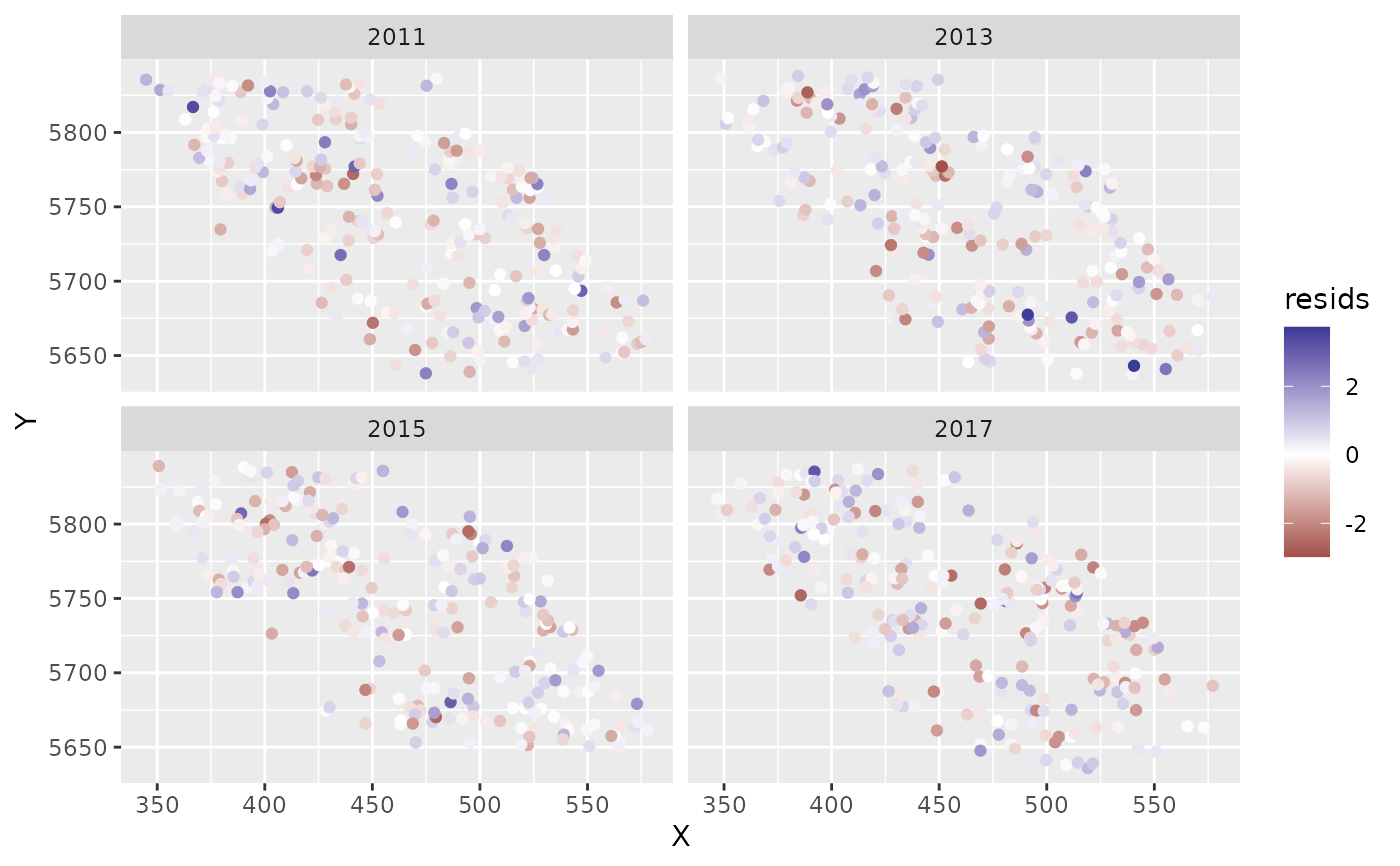
predictions$resids <- residuals(m) # randomized quantile residuals
library(ggplot2)
ggplot(predictions, aes(X, Y, col = resids)) + scale_colour_gradient2() +
geom_point() + facet_wrap(~year)
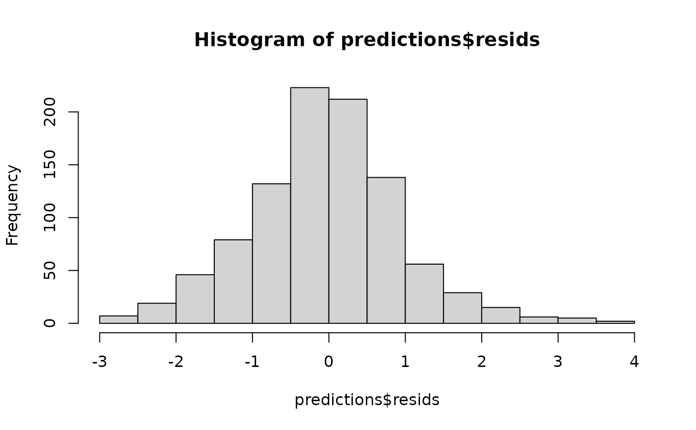
 hist(predictions$resids)
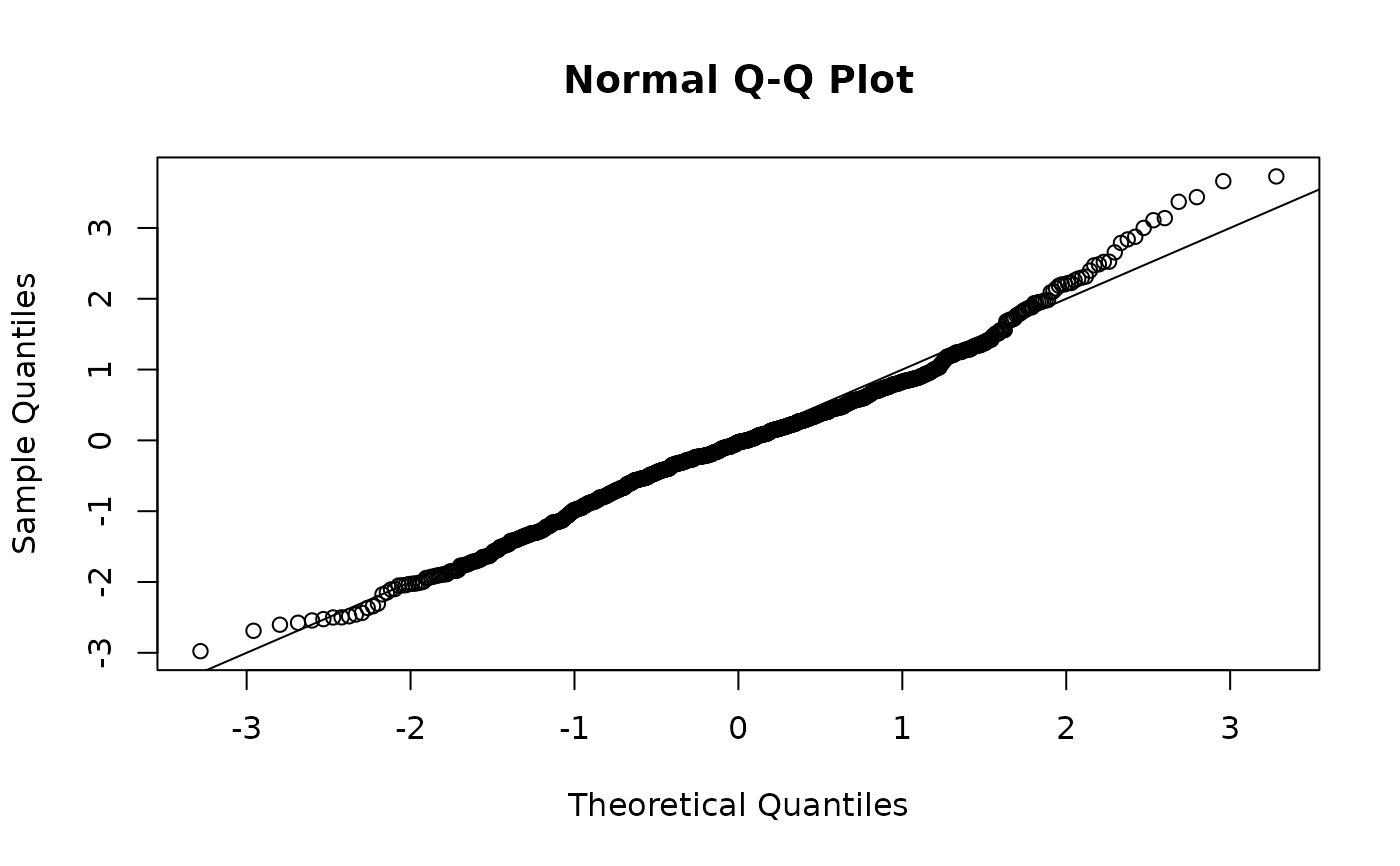
 qqnorm(predictions$resids); abline(a = 0, b = 1)
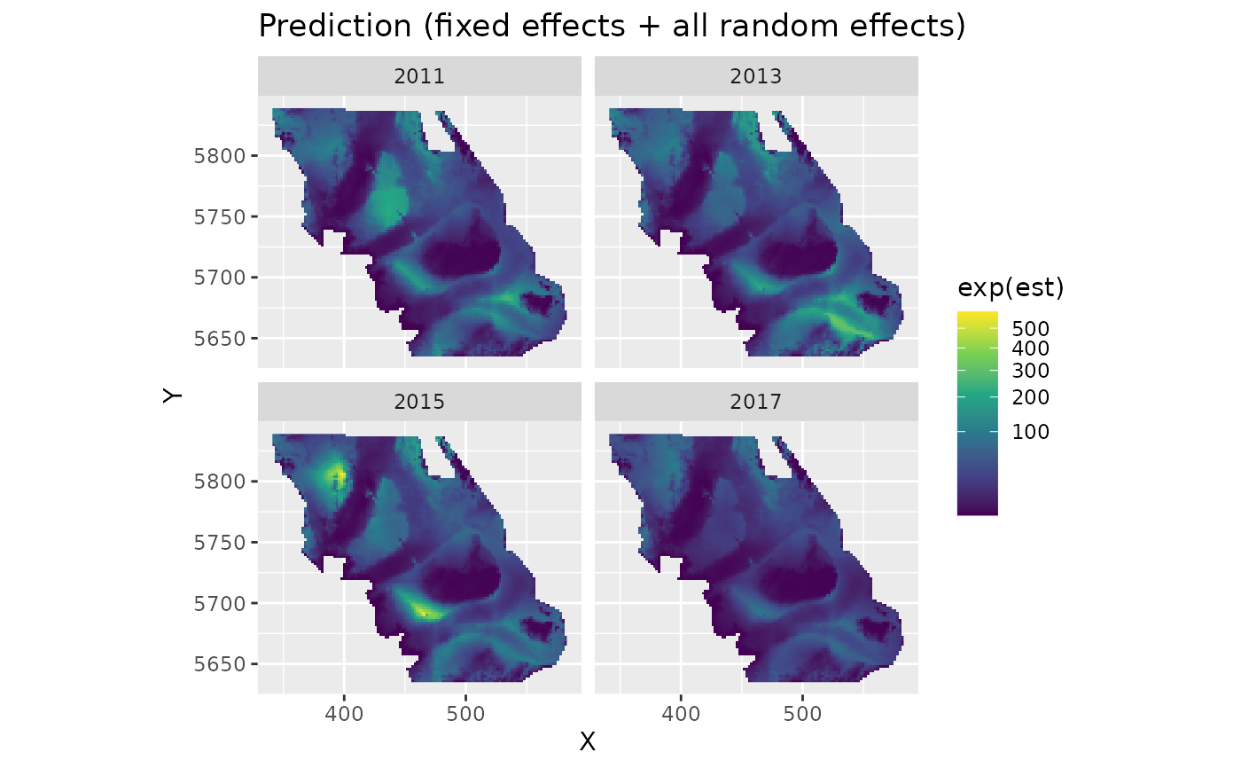
 # Predictions on new data ----------------------------------------------
qcs_grid_2011 <- replicate_df(qcs_grid, "year", unique(pcod_2011$year))
predictions <- predict(m, newdata = qcs_grid_2011)
# \donttest{
# A short function for plotting predictions:
plot_map <- function(dat, column = est) {
ggplot(dat, aes(X, Y, fill = {{ column }})) +
geom_raster() +
facet_wrap(~year) +
coord_fixed()
}
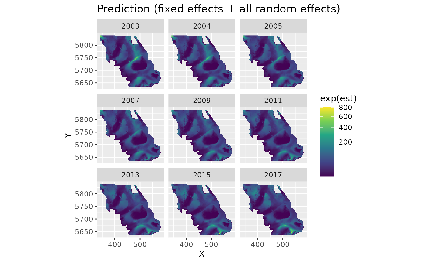
plot_map(predictions, exp(est)) +
scale_fill_viridis_c(trans = "sqrt") +
ggtitle("Prediction (fixed effects + all random effects)")
# Predictions on new data ----------------------------------------------
qcs_grid_2011 <- replicate_df(qcs_grid, "year", unique(pcod_2011$year))
predictions <- predict(m, newdata = qcs_grid_2011)
# \donttest{
# A short function for plotting predictions:
plot_map <- function(dat, column = est) {
ggplot(dat, aes(X, Y, fill = {{ column }})) +
geom_raster() +
facet_wrap(~year) +
coord_fixed()
}
plot_map(predictions, exp(est)) +
scale_fill_viridis_c(trans = "sqrt") +
ggtitle("Prediction (fixed effects + all random effects)")
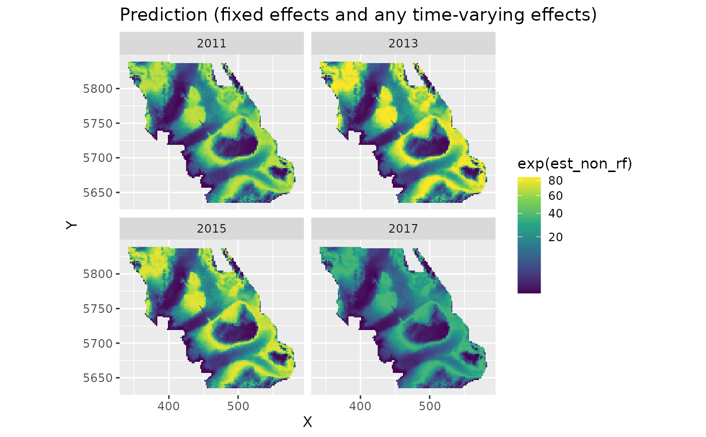
 plot_map(predictions, exp(est_non_rf)) +
ggtitle("Prediction (fixed effects and any time-varying effects)") +
scale_fill_viridis_c(trans = "sqrt")
plot_map(predictions, exp(est_non_rf)) +
ggtitle("Prediction (fixed effects and any time-varying effects)") +
scale_fill_viridis_c(trans = "sqrt")
 plot_map(predictions, est_rf) +
ggtitle("All random field estimates") +
scale_fill_gradient2()
plot_map(predictions, est_rf) +
ggtitle("All random field estimates") +
scale_fill_gradient2()
 plot_map(predictions, omega_s) +
ggtitle("Spatial random effects only") +
scale_fill_gradient2()
plot_map(predictions, omega_s) +
ggtitle("Spatial random effects only") +
scale_fill_gradient2()
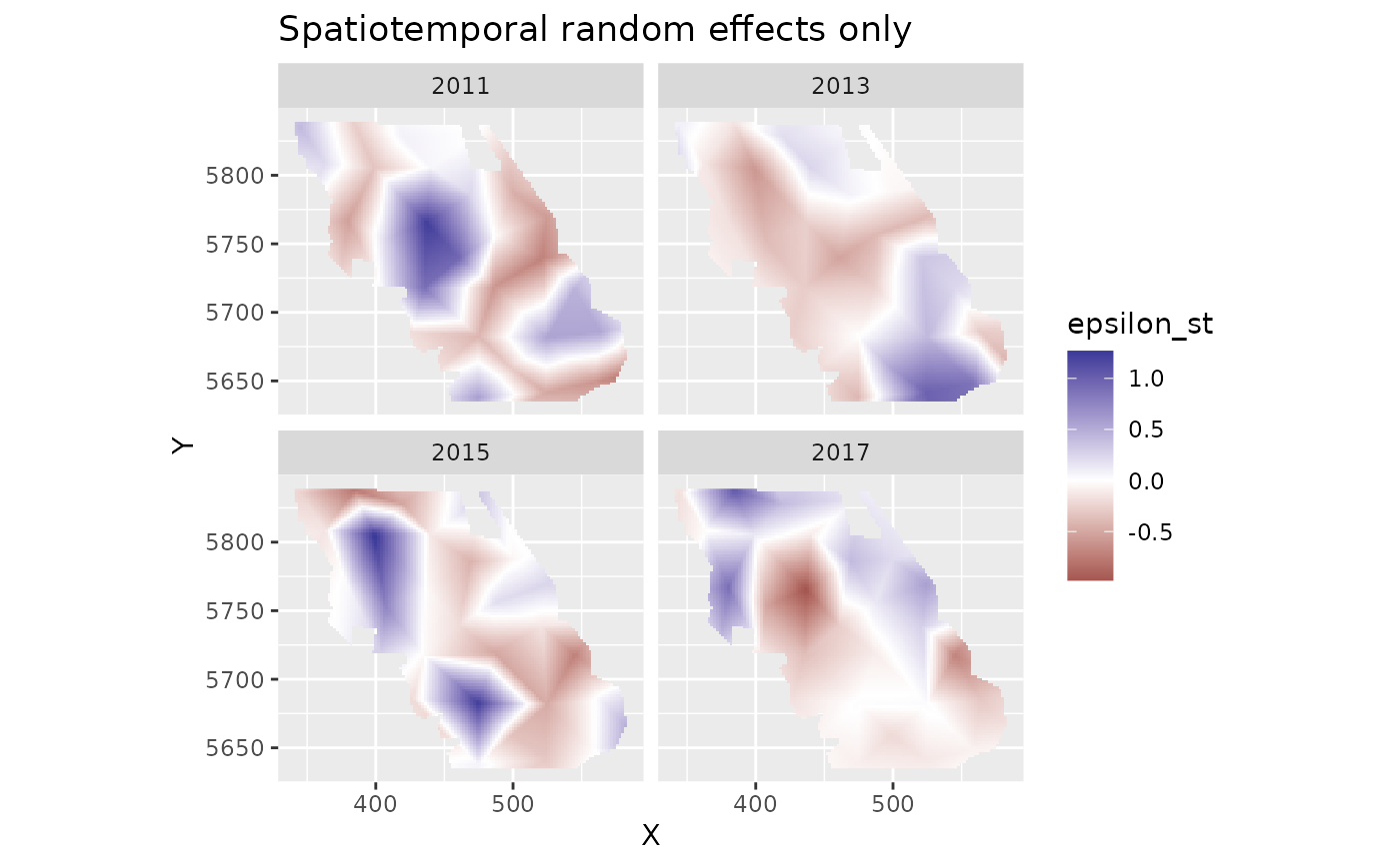
 plot_map(predictions, epsilon_st) +
ggtitle("Spatiotemporal random effects only") +
scale_fill_gradient2()
plot_map(predictions, epsilon_st) +
ggtitle("Spatiotemporal random effects only") +
scale_fill_gradient2()
 # Visualizing a marginal effect ----------------------------------------
# See the visreg package or the ggeffects::ggeffect() or
# ggeffects::ggpredict() functions
# To do this manually:
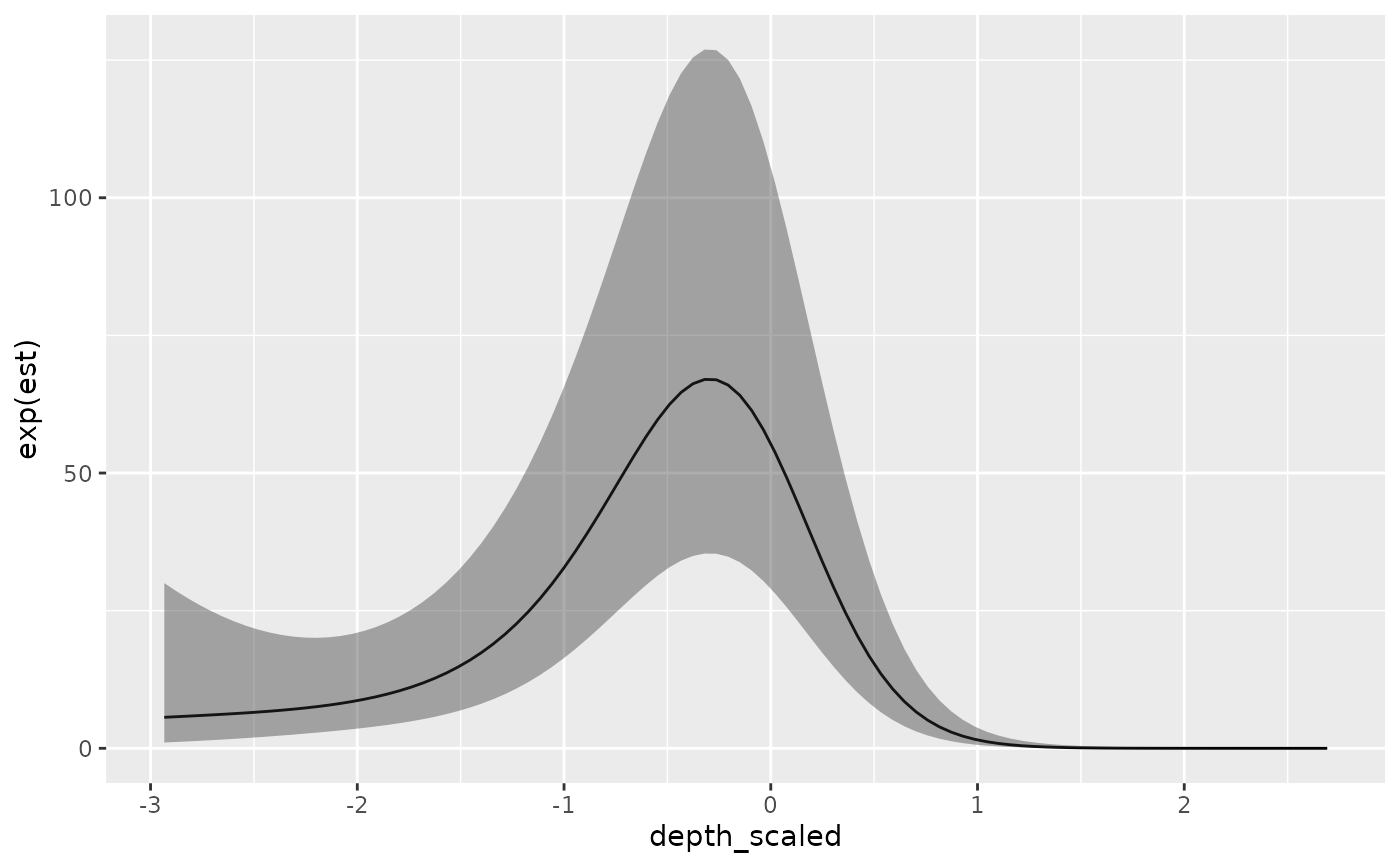
nd <- data.frame(depth_scaled =
seq(min(d$depth_scaled), max(d$depth_scaled), length.out = 100))
nd$depth_scaled2 <- nd$depth_scaled^2
# Because this is a spatiotemporal model, you'll need at least one time
# value. For these population-level predictions, if time isn't also a fixed
# effect, it doesn't matter what you pick:
nd$year <- 2011L # L: integer to match original data
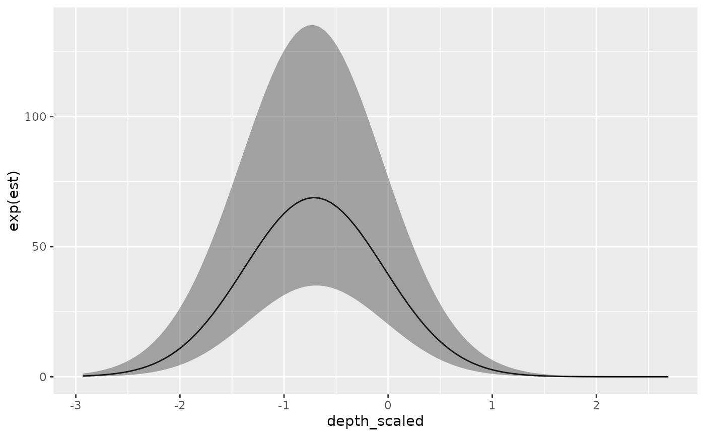
p <- predict(m, newdata = nd, se_fit = TRUE, re_form = NA)
ggplot(p, aes(depth_scaled, exp(est),
ymin = exp(est - 1.96 * est_se), ymax = exp(est + 1.96 * est_se))) +
geom_line() + geom_ribbon(alpha = 0.4)
# Visualizing a marginal effect ----------------------------------------
# See the visreg package or the ggeffects::ggeffect() or
# ggeffects::ggpredict() functions
# To do this manually:
nd <- data.frame(depth_scaled =
seq(min(d$depth_scaled), max(d$depth_scaled), length.out = 100))
nd$depth_scaled2 <- nd$depth_scaled^2
# Because this is a spatiotemporal model, you'll need at least one time
# value. For these population-level predictions, if time isn't also a fixed
# effect, it doesn't matter what you pick:
nd$year <- 2011L # L: integer to match original data
p <- predict(m, newdata = nd, se_fit = TRUE, re_form = NA)
ggplot(p, aes(depth_scaled, exp(est),
ymin = exp(est - 1.96 * est_se), ymax = exp(est + 1.96 * est_se))) +
geom_line() + geom_ribbon(alpha = 0.4)
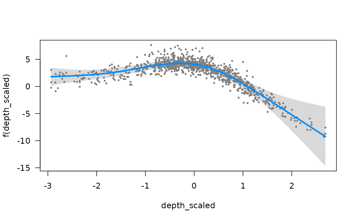
 # Plotting marginal effect of a spline ---------------------------------
m_gam <- sdmTMB(
data = d, formula = density ~ 0 + as.factor(year) + s(depth_scaled, k = 5),
time = "year", mesh = mesh, family = tweedie(link = "log")
)
if (require("visreg", quietly = TRUE)) {
visreg::visreg(m_gam, "depth_scaled")
}
# Plotting marginal effect of a spline ---------------------------------
m_gam <- sdmTMB(
data = d, formula = density ~ 0 + as.factor(year) + s(depth_scaled, k = 5),
time = "year", mesh = mesh, family = tweedie(link = "log")
)
if (require("visreg", quietly = TRUE)) {
visreg::visreg(m_gam, "depth_scaled")
}
 # or manually:
nd <- data.frame(depth_scaled =
seq(min(d$depth_scaled), max(d$depth_scaled), length.out = 100))
nd$year <- 2011L
p <- predict(m_gam, newdata = nd, se_fit = TRUE, re_form = NA)
ggplot(p, aes(depth_scaled, exp(est),
ymin = exp(est - 1.96 * est_se), ymax = exp(est + 1.96 * est_se))) +
geom_line() + geom_ribbon(alpha = 0.4)
# or manually:
nd <- data.frame(depth_scaled =
seq(min(d$depth_scaled), max(d$depth_scaled), length.out = 100))
nd$year <- 2011L
p <- predict(m_gam, newdata = nd, se_fit = TRUE, re_form = NA)
ggplot(p, aes(depth_scaled, exp(est),
ymin = exp(est - 1.96 * est_se), ymax = exp(est + 1.96 * est_se))) +
geom_line() + geom_ribbon(alpha = 0.4)
 # Forecasting ----------------------------------------------------------
mesh <- make_mesh(d, c("X", "Y"), cutoff = 15)
unique(d$year)
#> [1] 2011 2013 2015 2017
m <- sdmTMB(
data = d, formula = density ~ 1,
spatiotemporal = "AR1", # using AR(1) to have something to forecast with
extra_time = 2019L, # `L` for integer to match our data
spatial = "off",
time = "year", mesh = mesh, family = tweedie(link = "log")
)
# Add a year to our grid:
grid2019 <- qcs_grid_2011[qcs_grid_2011$year == max(qcs_grid_2011$year), ]
grid2019$year <- 2019L # `L` because `year` is an integer in the data
qcsgrid_forecast <- rbind(qcs_grid_2011, grid2019)
predictions <- predict(m, newdata = qcsgrid_forecast)
plot_map(predictions, exp(est)) +
scale_fill_viridis_c(trans = "log10")
# Forecasting ----------------------------------------------------------
mesh <- make_mesh(d, c("X", "Y"), cutoff = 15)
unique(d$year)
#> [1] 2011 2013 2015 2017
m <- sdmTMB(
data = d, formula = density ~ 1,
spatiotemporal = "AR1", # using AR(1) to have something to forecast with
extra_time = 2019L, # `L` for integer to match our data
spatial = "off",
time = "year", mesh = mesh, family = tweedie(link = "log")
)
# Add a year to our grid:
grid2019 <- qcs_grid_2011[qcs_grid_2011$year == max(qcs_grid_2011$year), ]
grid2019$year <- 2019L # `L` because `year` is an integer in the data
qcsgrid_forecast <- rbind(qcs_grid_2011, grid2019)
predictions <- predict(m, newdata = qcsgrid_forecast)
plot_map(predictions, exp(est)) +
scale_fill_viridis_c(trans = "log10")
 plot_map(predictions, epsilon_st) +
scale_fill_gradient2()
plot_map(predictions, epsilon_st) +
scale_fill_gradient2()
 # Estimating local trends ----------------------------------------------
d <- pcod
d$year_scaled <- as.numeric(scale(d$year))
mesh <- make_mesh(pcod, c("X", "Y"), cutoff = 25)
m <- sdmTMB(data = d, formula = density ~ depth_scaled + depth_scaled2,
mesh = mesh, family = tweedie(link = "log"),
spatial_varying = ~ 0 + year_scaled, time = "year", spatiotemporal = "off")
nd <- replicate_df(qcs_grid, "year", unique(pcod$year))
nd$year_scaled <- (nd$year - mean(d$year)) / sd(d$year)
p <- predict(m, newdata = nd)
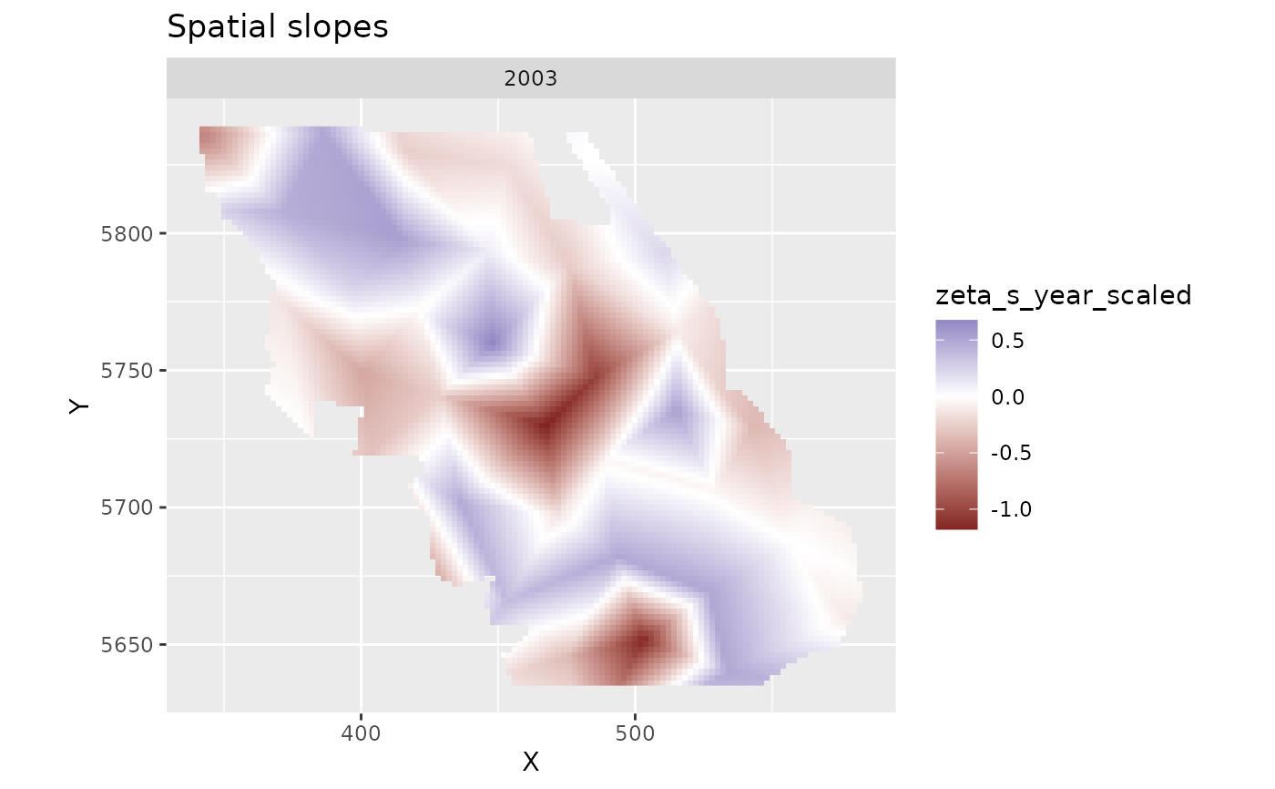
plot_map(subset(p, year == 2003), zeta_s_year_scaled) + # pick any year
ggtitle("Spatial slopes") +
scale_fill_gradient2()
# Estimating local trends ----------------------------------------------
d <- pcod
d$year_scaled <- as.numeric(scale(d$year))
mesh <- make_mesh(pcod, c("X", "Y"), cutoff = 25)
m <- sdmTMB(data = d, formula = density ~ depth_scaled + depth_scaled2,
mesh = mesh, family = tweedie(link = "log"),
spatial_varying = ~ 0 + year_scaled, time = "year", spatiotemporal = "off")
nd <- replicate_df(qcs_grid, "year", unique(pcod$year))
nd$year_scaled <- (nd$year - mean(d$year)) / sd(d$year)
p <- predict(m, newdata = nd)
plot_map(subset(p, year == 2003), zeta_s_year_scaled) + # pick any year
ggtitle("Spatial slopes") +
scale_fill_gradient2()
 plot_map(p, est_rf) +
ggtitle("Random field estimates") +
scale_fill_gradient2()
plot_map(p, est_rf) +
ggtitle("Random field estimates") +
scale_fill_gradient2()
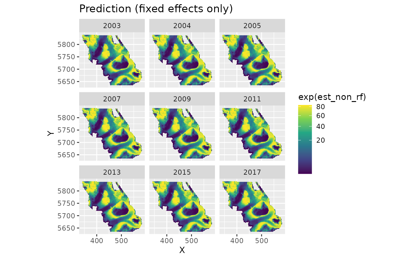
 plot_map(p, exp(est_non_rf)) +
ggtitle("Prediction (fixed effects only)") +
scale_fill_viridis_c(trans = "sqrt")
plot_map(p, exp(est_non_rf)) +
ggtitle("Prediction (fixed effects only)") +
scale_fill_viridis_c(trans = "sqrt")
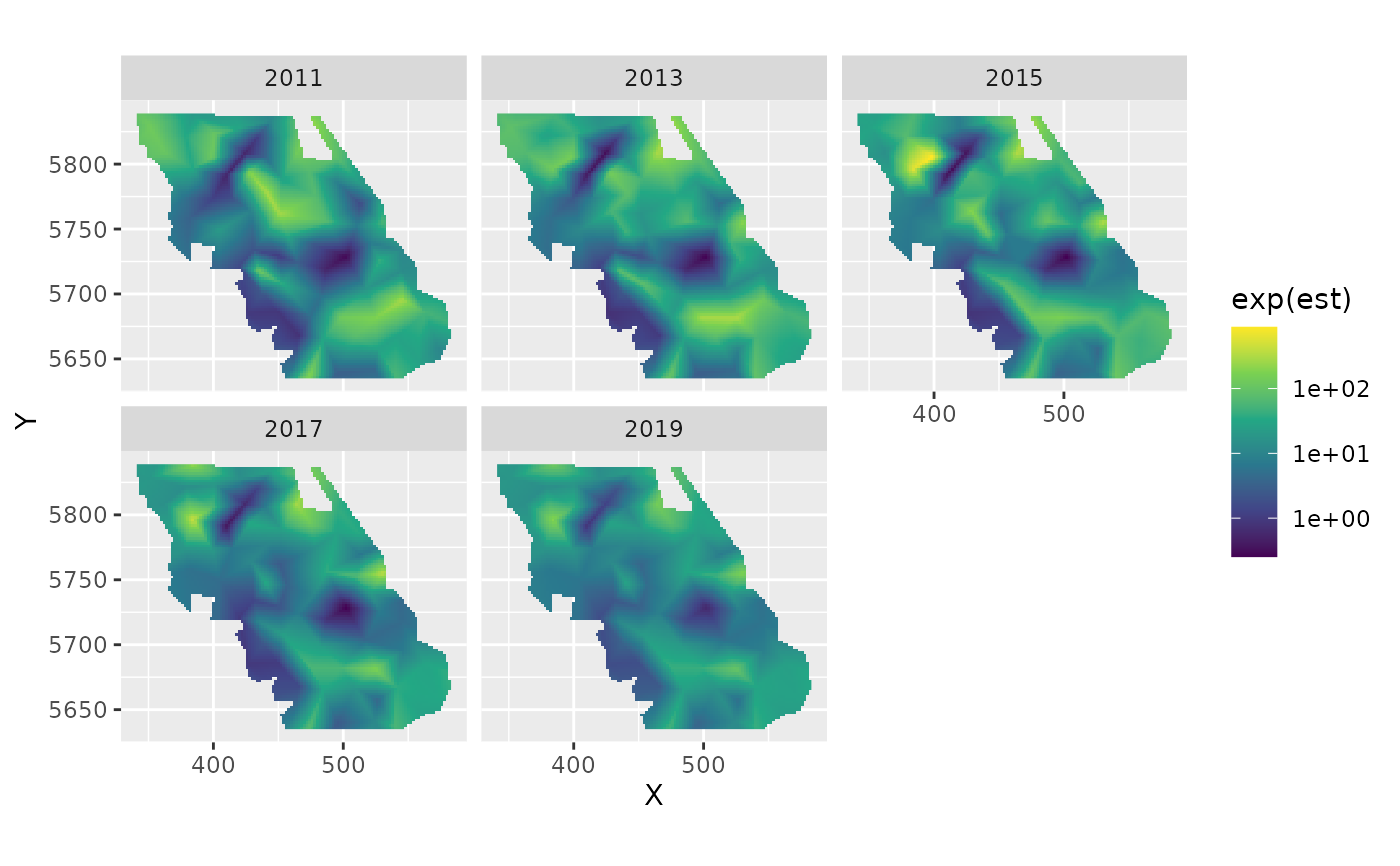
 plot_map(p, exp(est)) +
ggtitle("Prediction (fixed effects + all random effects)") +
scale_fill_viridis_c(trans = "sqrt")
plot_map(p, exp(est)) +
ggtitle("Prediction (fixed effects + all random effects)") +
scale_fill_viridis_c(trans = "sqrt")
 # }
# }