Poisson-link delta models

Introduction

Jim Thorson introduced the Poisson-link delta model in a CJFAS paper (Thorson 2018). It is a useful model family when dealing with positive continuous data that have zeros. It can be used in the same circumstances that you could use the Tweedie or a traditional delta-gamma or delta-lognormal model with logit and log links.

The Poisson-link delta formulation describes how to go from linear predictors in link space to expected values that enter the data likelihood. The likelihood for the first component is Bernoulli (i.e., binomial with a single trial), and the likelihood for the second component can be gamma or lognormal.

In sdmTMB, these families are specified as delta_gamma(type = "poisson-link") and delta_lognormal(type = "poisson-link").

The model

Thorson (2018) describes the process model as:

$$\begin{aligned} p &= 1 - \exp(-n),\\ r &= \frac{n w}{p}, \end{aligned}$$ where $p$ represents encounter probability, $n$ represents group numbers density, $r$ represents positive catch rate (i.e., catch rate given encounter), and $w$ represents weight per group.

The linear predictors represent log group numbers density ($\log (n)$) and log weight per group ($\log (w)$):

$$\begin{aligned} \log (n) &= \boldsymbol{X_1} \boldsymbol{\beta_1} + \ldots,\\ \log (w) &= \boldsymbol{X_2} \boldsymbol{\beta_2} + \ldots, \end{aligned}$$

where the $\boldsymbol{X}$s represent design matrices, the $\boldsymbol{\beta}$s represent coefficient vectors, and the $\ldots$ represents all other possible model components that are linear in link space, including any random fields.

These are transformed with the above process equations to generate $p$ and $r$. Then the model evaluates the following likelihood components. For the encounter probability $p$

$$\operatorname{Bernoulli} (p),$$

or equivalently

$$\operatorname{Binomial} (1, p),$$

and for the positive rate $r$, either the gamma or lognormal likelihood

$$\operatorname{Gamma} \left( \phi, \frac{r}{\phi} \right),$$ where $\phi$ represents the gamma shape and $r / \phi$ represents the scale, or

$$\operatorname{Lognormal} \left( \log (r) - \frac{\phi^2}{2}, \phi^2 \right),$$

where $\log (r) - \frac{\phi^2}{2}$ represents the bias-corrected log mean and $\phi$ represents the standard deviation in log-space.

An example

Data

We will work with Pacific Spiny Dogfish observations from a trawl survey off the west coast of Vancouver Island, Canada. The dataset dogfish is included in the sdmTMB package.

library(ggplot2)
theme_set(theme_light())
library(dplyr)
library(sdmTMB)

dogfish$log_depth <- log(dogfish$depth)
head(dogfish)
#> # A tibble: 6 × 10
#>    year longitude latitude     X     Y present catch_weight area_swept depth
#>   <int>     <dbl>    <dbl> <dbl> <dbl>   <int>        <dbl>      <dbl> <dbl>
#> 1  2004     -125.     48.7  780. 5399.       1         22.7     0.103     73
#> 2  2004     -126.     48.2  735. 5346.       0          0       0.103    455
#> 3  2004     -126.     48.3  738. 5355.       0          0       0.116    171
#> 4  2004     -126.     48.3  749. 5354.       1        221.      0.122    137
#> 5  2004     -126.     48.4  744. 5362.       1        440.      0.0964   140
#> 6  2004     -126.     48.4  737. 5362.       1         48.2     0.122    145
#> # ℹ 1 more variable: log_depth <dbl>

mesh <- make_mesh(dogfish, c("X", "Y"), cutoff = 10)

A conventional delta-gamma model:

First, let’s fit a conventional delta-gamma model with logit and log links and illustrate a limitation.

fit_dg <- sdmTMB(catch_weight ~ 0 + as.factor(year) + s(log_depth),
  family = delta_gamma(),
  spatial = "on",
  mesh = mesh,
  data = dogfish,
  anisotropy = FALSE,
  reml = TRUE,
  offset = log(dogfish$area_swept),
  silent = FALSE
)

sanity(fit_dg)
#> ✔ Non-linear minimizer suggests successful convergence
#> ✔ Hessian matrix is positive definite
#> ✔ No extreme or very small eigenvalues detected
#> ✔ No gradients with respect to fixed effects are >= 0.001
#> ✔ No fixed-effect standard errors are NA
#> ✔ No standard errors look unreasonably large
#> ✔ No sigma parameters are < 0.01
#> ✔ No sigma parameters are > 100
#> ✔ Range parameters don't look unreasonably large

How can we show the effect of depth on catch weight? There is no single curve, because the two components use different links (logit + log), so the relationship between catch weight and depth depends on the expected catch weight implied by the other coefficients (here, year, but also location in space because of the spatial random field).

For example, here is how the curves look for different years:

nd <- expand.grid(
  log_depth = seq(min(dogfish$log_depth), max(dogfish$log_depth), length.out = 200),
  year = as.factor(unique(dogfish$year))
)
p <- predict(fit_dg, newdata = nd, re_form = NA)
ggplot(p, aes(log_depth, log(plogis(est1) * exp(est2)), colour = year)) +
  geom_line() +
  ylab("log expected catch weight")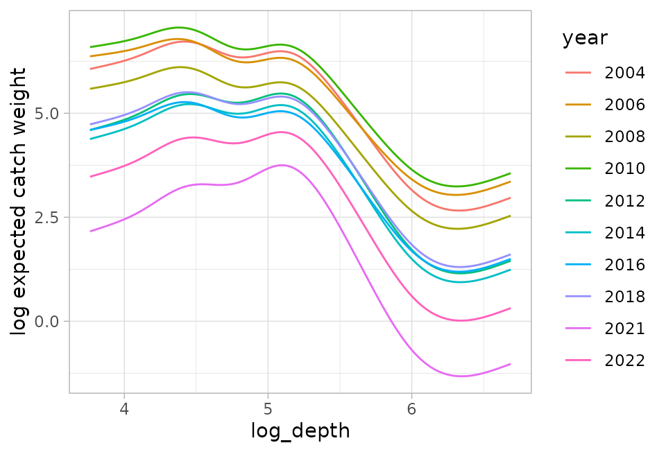

There is no one curve! It depends on the value of year.

A Poisson-link-delta-gamma alternative

Instead, let’s fit a Poisson-link delta-gamma model:

fit_dpg <- sdmTMB(catch_weight ~ 0 + as.factor(year) + s(log_depth),
  family = delta_gamma(type = "poisson-link"),
  spatial = "on",
  mesh = mesh,
  data = dogfish,
  anisotropy = TRUE,
  reml = TRUE,
  offset = log(dogfish$area_swept),
  silent = FALSE
)

sanity(fit_dpg)
#> ✔ Non-linear minimizer suggests successful convergence
#> ✔ Hessian matrix is positive definite
#> ✔ No extreme or very small eigenvalues detected
#> ✔ No gradients with respect to fixed effects are >= 0.001
#> ✔ No fixed-effect standard errors are NA
#> ✔ No standard errors look unreasonably large
#> ✔ No sigma parameters are < 0.01
#> ✔ No sigma parameters are > 100
summary(fit_dpg)
#> Spatial model fit by REML ['sdmTMB']
#> Formula: catch_weight ~ 0 + as.factor(year) + s(log_depth)
#> Mesh: mesh (anisotropic covariance)
#> Data: dogfish
#> Family: delta_gamma(link1 = 'log', link2 = 'log', type = 'poisson-link')
#> 
#> Delta/hurdle model 1: -----------------------------------
#> Family: binomial(link = 'log') 
#> Conditional model:
#>                     coef.est coef.se
#> as.factor(year)2004     1.96    0.77
#> as.factor(year)2006     2.89    0.77
#> as.factor(year)2008     2.57    0.76
#> as.factor(year)2010     2.43    0.77
#> as.factor(year)2012     1.94    0.76
#> as.factor(year)2014     1.93    0.76
#> as.factor(year)2016     2.20    0.76
#> as.factor(year)2018     2.03    0.76
#> as.factor(year)2021     1.18    0.76
#> as.factor(year)2022     1.75    0.76
#> slog_depth              0.15    0.54
#> 
#> Smooth terms:
#>                  Std. Dev.
#> sd__s(log_depth)      2.38
#> 
#> Matérn anisotropic range (spatial): 26.1 to 381.1 at 142 deg.
#> Spatial SD: 1.18
#> 
#> Delta/hurdle model 2: -----------------------------------
#> Family: Gamma(link = 'log') 
#> Conditional model:
#>                     coef.est coef.se
#> as.factor(year)2004     3.59    0.37
#> as.factor(year)2006     2.78    0.33
#> as.factor(year)2008     2.47    0.32
#> as.factor(year)2010     3.50    0.34
#> as.factor(year)2012     2.77    0.33
#> as.factor(year)2014     2.45    0.33
#> as.factor(year)2016     2.09    0.32
#> as.factor(year)2018     2.60    0.32
#> as.factor(year)2021     1.69    0.33
#> as.factor(year)2022     1.98    0.33
#> slog_depth             -0.20    0.82
#> 
#> Smooth terms:
#>                  Std. Dev.
#> sd__s(log_depth)      5.09
#> 
#> Dispersion parameter: 0.59
#> Matérn anisotropic range (spatial): 4.2 to 60.8 at 142 deg.
#> Spatial SD: 1.97
#> 
#> REML criterion at convergence: 5851.613
#> 
#> See ?tidy.sdmTMB to extract these values as a data frame.
#> See ?plot_anisotropy to plot the anisotropic range.

and make the same plot:

p_dpg <- predict(fit_dpg, newdata = nd, re_form = NA)
ggplot(p_dpg, aes(log_depth, est1 + est2, colour = year)) +
  geom_line() +
  ylab("log expected catch weight")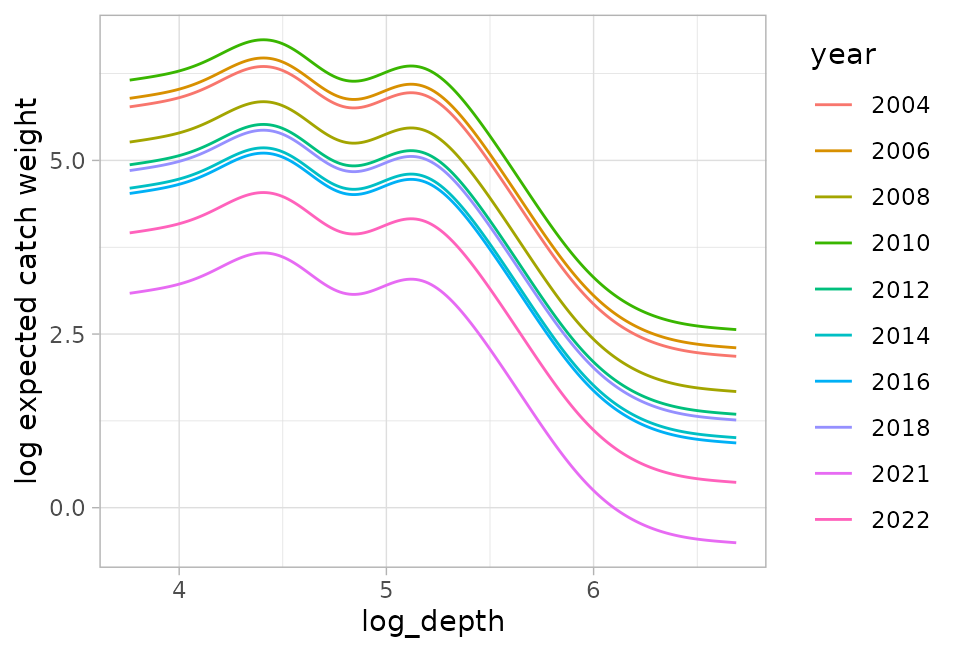

Note how the lines are now parallel. Other predictors shift the curve up and down but do not affect the shape of the combined prediction because both components use a log link.

Examining the model components and how they combine

We’ll make some predictions across depths but for a single year for simplicity:

nd2010 <- dplyr::filter(nd, year == 2010)
p_pdg <- predict(fit_dpg, newdata = nd2010, re_form = NA)

We can extract the components of our theoretical decomposition of catch into group numbers density, weight per group, encounter probability, and positive rate:

n <- exp(p_pdg$est1)
w <- exp(p_pdg$est2)
p <- 1 - exp(-n)
r <- (n * w) / p

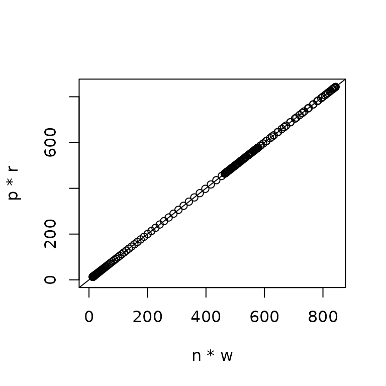
We can come up with our overall predictions in two ways:

1. n * w: group numbers $\times$ weight per group. This is equivalently exp(est1 + est2), where est1 and est2 are the linear predictors in link space.

2. p * r: encounter probability $\times$ positive catch rate.

These give identical answers:

lims <- c(0, max(p * r))
plot(n * w, p * r, xlim = lims, ylim = lims)
abline(0, 1)

Let’s plot out all the components and possible combinations:

g1 <- ggplot(p_pdg, aes(log_depth, n)) +
  geom_line() +
  ggtitle("Expected group density")
g2 <- ggplot(p_pdg, aes(log_depth, w)) +
  geom_line() +
  ggtitle("Expected weight per group")
g3 <- ggplot(p_pdg, aes(log_depth, p)) +
  geom_line() +
  ylim(0, 1) +
  ggtitle("Expected encounter probability")
g4 <- ggplot(p_pdg, aes(log_depth, r)) +
  geom_line() +
  ggtitle("Expected catch given encounter")
g5 <- ggplot(p_pdg, aes(log_depth, n * w)) +
  geom_line() +
  ggtitle("Expected catch")
g6 <- ggplot(p_pdg, aes(log_depth, p * r)) +
  geom_line() +
  ggtitle("Expected catch")

cowplot::plot_grid(g1, g2, g3, g4, g5, g6, ncol = 2)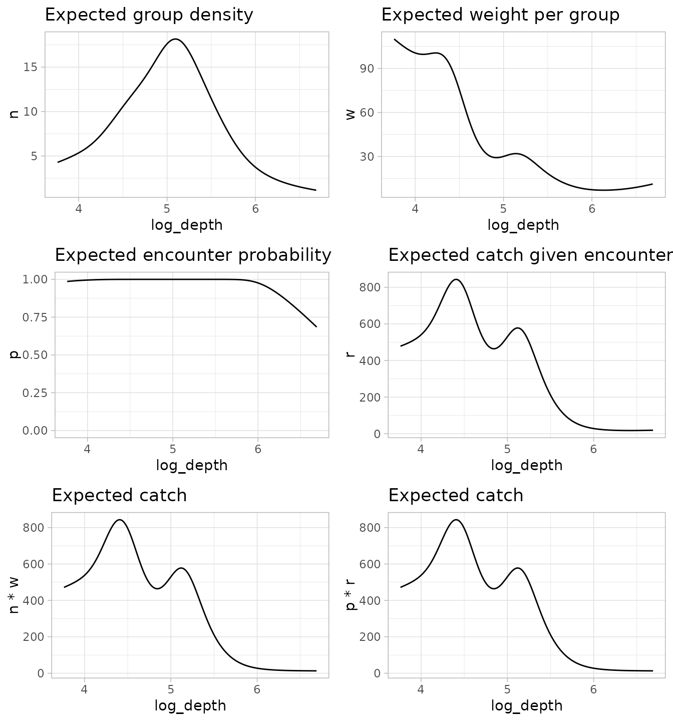

FAQ

What is a ‘group’ and how does the model know about numbers?

The model represents a process in which groups of fish (or other observations, of course) are encountered in certain numbers (“group numbers density”), and each group has a certain weight (“weight per group”).

This is a theoretical construct reflecting how the model can best parse the two components given the properties of the observed data. Since the predicted response value is $n \cdot w$, you can arrive at the same value by multiplying $n$ and dividing $w$ by the same amount. You could have more groups and less weight per group, or fewer groups and more weight per group, and arrive at the same expected catch. However, there is a balance of the two, given covariates and random effects, that best fits the data when entered into the likelihood as $p$ and $r$.

What is the connection to the complementary log-log link (‘cloglog’) and the Poisson?

From Wikipedia: “The cloglog model corresponds to applications where we observe either zero events (e.g., defects) or one or more, where the number of events is assumed to follow the Poisson distribution.” The explanation below is based on that idea.

Under a Poisson model, the probability of observing a zero given expected number $n$ is $\exp(-n)$. That is,

$$\mathrm{Pr}(0) = \exp(-n)$$ If $p$ is the probability of observing a non-zero (i.e., an encounter), then

$$\exp(-n) = 1 - p = \mathrm{Pr}(0).$$

We can re-arrange that as

$$n = -\log(1 - p).$$

And since we want our linear predictor to take values from negative to positive infinity (and therefore keep predicted number densities positive after exponentiating), we work in log space:

$$\log (n) = \log(-\log(1 - p)).$$

The right side is known as the ‘cloglog’ link function.

This link has the following inverse link function:

$$p = 1 - \exp(-\exp(\log n)).$$

We can check this in R:

p <- 0.78
log_n <- log(-log(1 - p))
log_n
#> [1] 0.4148395
1 - exp(-exp(log_n))
#> [1] 0.78

You can see that the cloglog inverse link is the same as the first part of our Poisson-link delta model. However, the ‘trick’ here is that group density $n$ affects both encounter probability $p$ (as shown above) and positive catch rates $r$:

$$r = \frac{n w}{p}.$$

So, when going from the linear predictors (which have log links) to the expected values entering the data likelihood (binomial + lognormal/gamma), the first linear predictor plays double duty in that it appears in both delta-model expected values.

What are the advantages of using such a model?

1. The Poisson-link families have the flexibility of a delta model, which in practice is often helpful for prediction. This could be checked with AIC or, better yet, cross-validation.

2. Like other delta models, there is a decomposition of the process into two theoretical parts. This can help interpretation (or make it more complicated!). Here, these parts can be rearranged to represent two ways of thinking about the same two components ($n$ and $w$, or $p$ and $r$).

3. Compared to a traditional delta-gamma model that has a logit and log link, the two linear predictors both have log links, so their coefficients are interpretable as multiplicative effects, and their effects can be combined. For example, their coefficients can be added in log space, and their predictions can be added in log space to generate a single response curve for a given predictor.

Where does the offset come in?

The offset is added to the linear predictor for $\log n$, i.e., as exp(offset) * n. For example, if $a$ represents area swept (a measure of effort) and log area swept is entered into the model as the offset, then

$$p = 1 - \exp(-a \cdot n).$$

Therefore, the encounter probability goes to 1 as area swept (effort) and underlying group numbers density increase toward infinity. This carries over to the positive rate $r$ via $p$ because $r = nw/p$.

Why call it a Poisson-link?

I can only guess. The cloglog function is derived from Poisson theory, and although the cloglog function appears in the Poisson-link model, the interaction of the two model components makes it different from a simple cloglog model, so I assume it needed another name.

These equations don’t look anything like the sdmTMB source code!

That is because the calculations have to be done in log space for computational stability, and some calculations are fastest and most stable if implemented slightly differently from how they are most naturally described in the equations above.

References

Thorson, J.T. (2018). Three problems with the conventional delta-model for biomass sampling data, and a computationally efficient alternative. Canadian Journal of Fisheries and Aquatic Sciences, 75, 1369–1382.