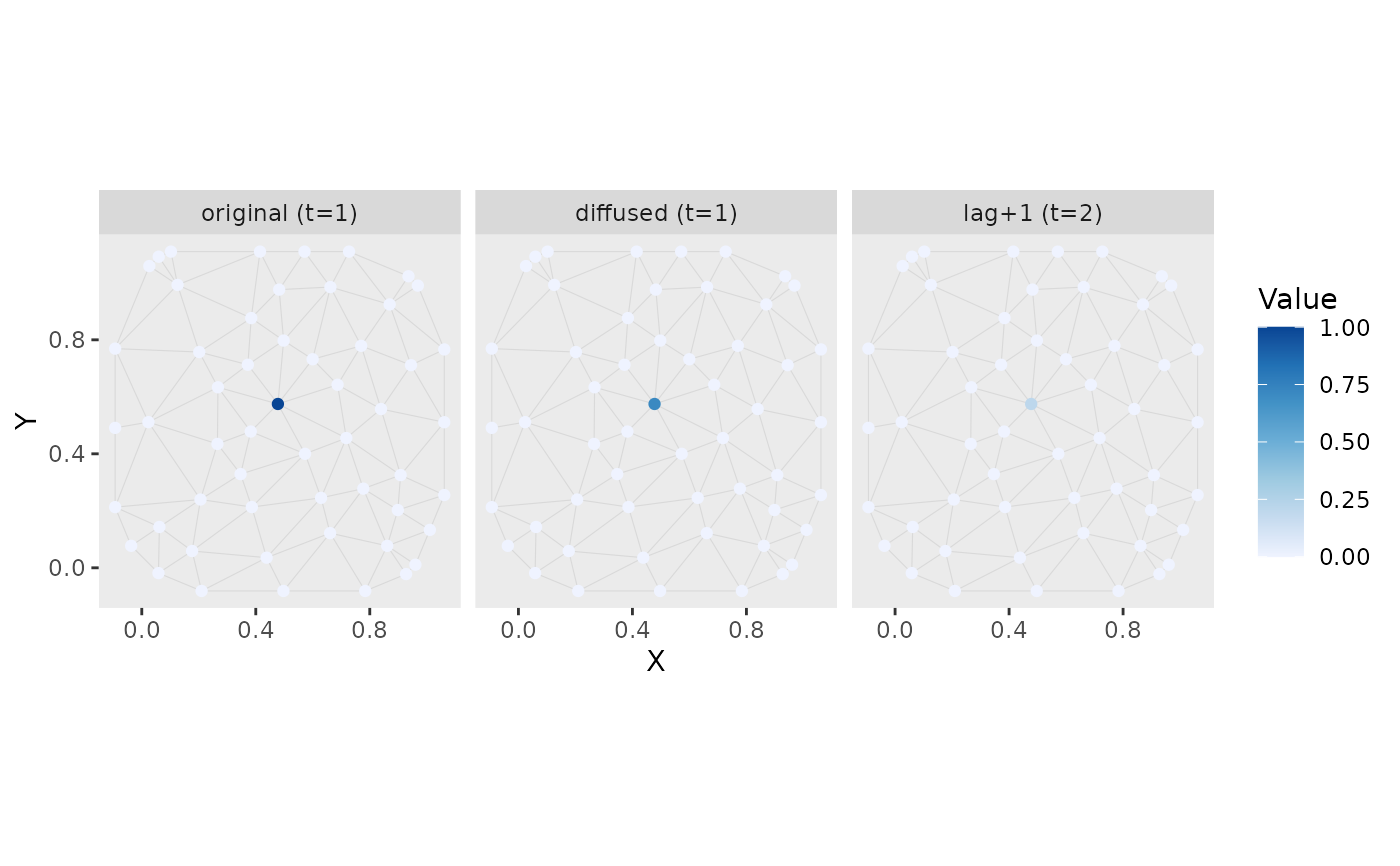
Plot Covariate-Diffusion Diagnostics — plot_nonlocal

Visualize fitted covariate-diffusion transforms or impulse-response kernels for one selected covariate-diffusion term. By default, values are plotted at mesh vertices with the mesh edges shown in light grey. Values can also be evaluated at supplied newdata coordinates and plotted as points or a raster.

Usage

plot_nonlocal_covariate(
  object,
  component,
  newdata = NULL,
  type = c("point", "raster"),
  covariate = NULL,
  time_value = 1,
  n_steps = 1L,
  common_scale = TRUE
)

plot_nonlocal_kernel(
  object,
  component,
  newdata = NULL,
  type = c("point", "raster"),
  covariate = NULL,
  time_value = 1,
  n_steps = 3L,
  common_scale = FALSE
)

Arguments

object: A fitted sdmTMB() model with nonlocal_formula.
component: Covariate-diffusion component name. Must be one of "diffusion", "time_lag", or "combined". "combined" plots the joint response of all covariate-diffusion components fitted for covariate.
newdata: Optional data frame with x/y coordinate columns matching the fitted mesh. If supplied, values are evaluated at the unique newdata coordinates. If NULL, values are evaluated at mesh vertices.
type: Plot type: "point" or "raster". "raster" requires newdata.
covariate: Optional covariate name from nonlocal_formula. Required when multiple lag covariates were fitted.
time_value: Optional time slice to plot or use for the impulse. Supply either a modeled time value or a 1-based time index. Defaults to 1.
n_steps: Number of transformed slices to plot starting at time_value.
common_scale: Should the plotted panels share a common color scale? Defaults to TRUE for plot_nonlocal_covariate() and FALSE for plot_nonlocal_kernel(). component = "time_lag" alone likely needs common_scale = TRUE to make sense.

Value

A ggplot object.

Details

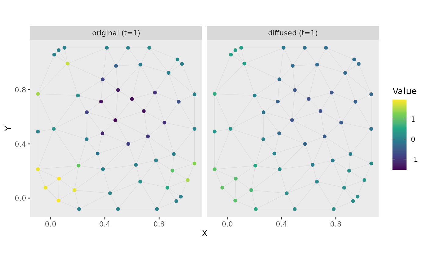
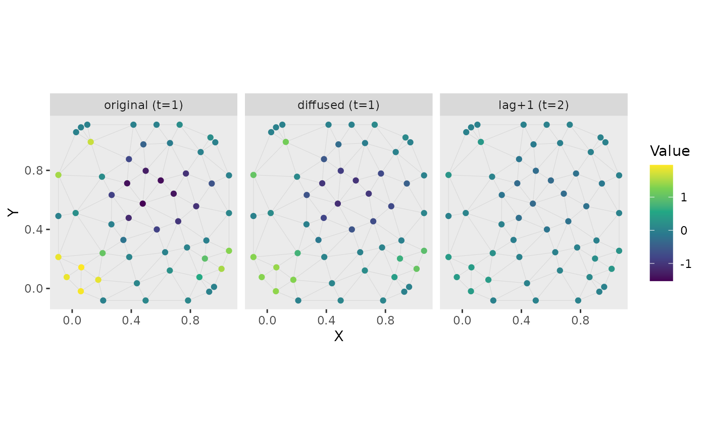
plot_nonlocal_covariate() visualizes the original mesh-vertex covariate field and its fitted covariate-diffusion transform for one selected covariate time slice across one or more lagged output time slices.

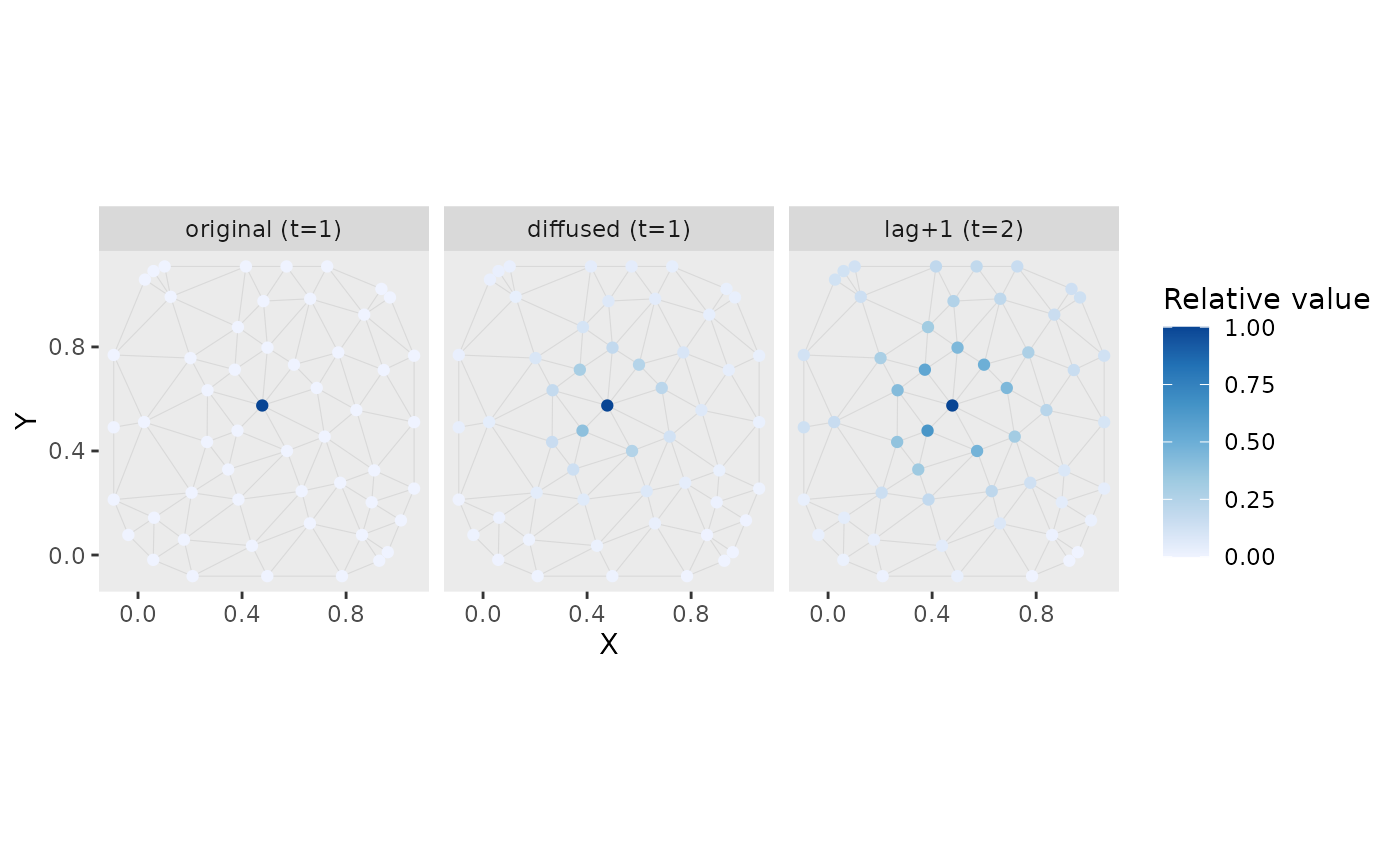
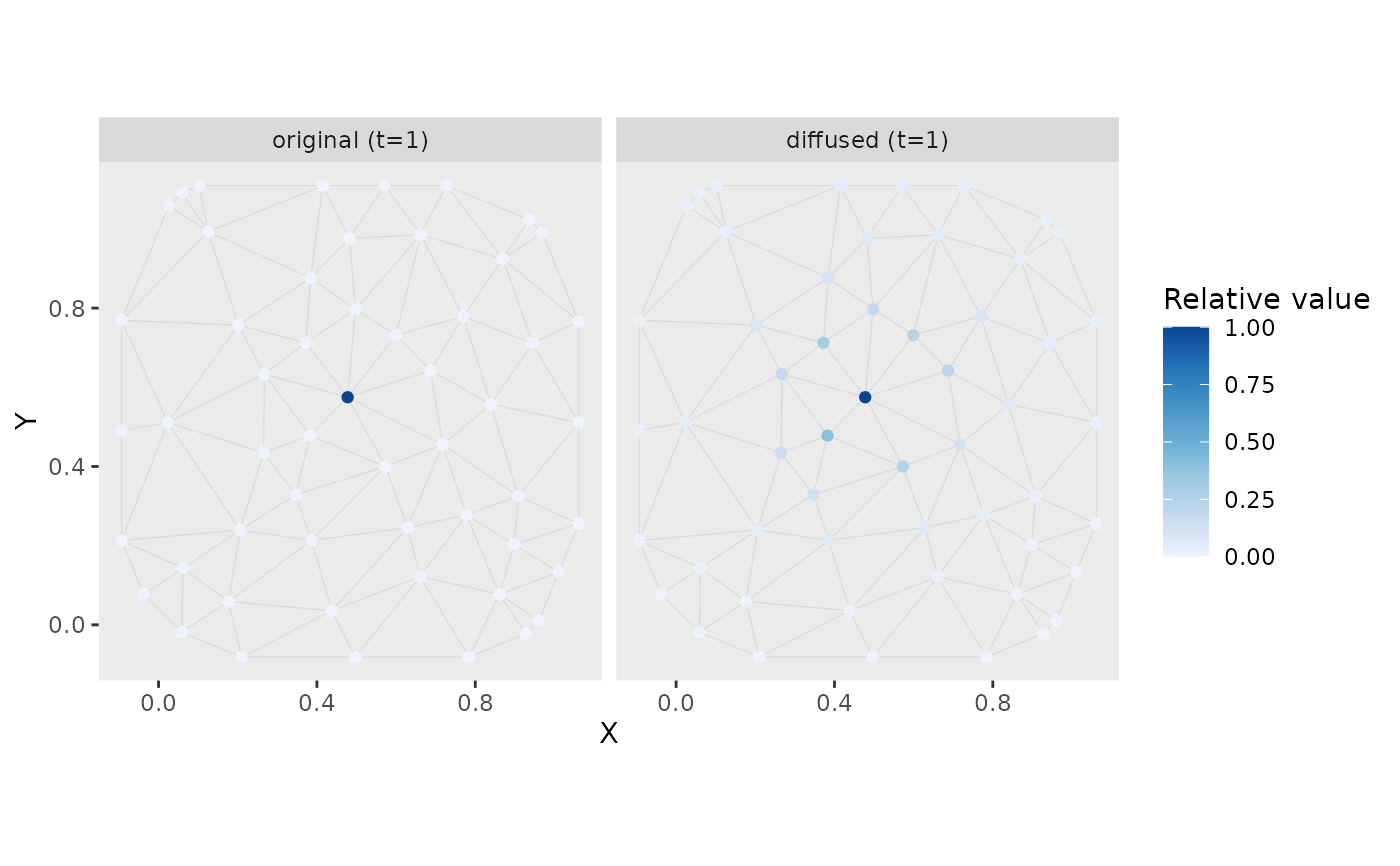
plot_nonlocal_kernel() visualizes an impulse entering and diffusing through one covariate-diffusion component.

Examples


# Simulate some data for fitting:
set.seed(1)
n_t <- 6
n_sites <- 80
sites <- data.frame(X = runif(n_sites), Y = runif(n_sites))
dat <- data.frame(
  X = rep(sites$X, times = n_t),
  Y = rep(sites$Y, times = n_t),
  year = rep(seq_len(n_t), each = n_sites)
)
dat$x1 <- as.numeric(scale(
  sin(2 * pi * (dat$X + dat$year / 6)) +
    cos(2 * pi * (dat$Y - dat$year / 8)) +
    0.4 * sin(4 * pi * dat$X) * cos(dat$year / 2) +
    rnorm(nrow(dat), sd = 0.15)
))
mesh <- make_mesh(dat, xy_cols = c("X", "Y"), cutoff = 0.12)
sim <- simulate_new(
  formula = ~ 1,
  data = dat,
  mesh = mesh,
  time = "year",
  family = gaussian(),
  spatial = "off",
  spatiotemporal = "off",
  range = 0.3,
  sigma_O = 0,
  sigma_E = 0,
  phi = 0.1,
  B = c(0, 0.7, 0.6),
  nonlocal_formula = ~ diffusion(x1) + time_lag(x1),
  lags_kappaS = 4.4,
  lags_rhoT = 0.3,
  seed = 123
)
dat$observed <- sim$observed

# Fit the model:
fit <- sdmTMB(
  observed ~ 1,
  data = dat,
  mesh = mesh,
  time = "year",
  spatial = "off", # keeping example simple
  spatiotemporal = "off", # keeping example simple
  family = gaussian(),
  nonlocal_formula = ~ diffusion(x1) + time_lag(x1) #<
)

plot_nonlocal_covariate(
  fit,
  covariate = "x1",
  component = "diffusion"
)

plot_nonlocal_covariate(
  fit,
  covariate = "x1",
  component = "time_lag",
  time_value = 1,
  n_steps = 2
)

plot_nonlocal_covariate(
  fit,
  covariate = "x1",
  component = "combined",
  time_value = 1,
  n_steps = 2
)

plot_nonlocal_kernel(
  fit,
  covariate = "x1",
  component = "diffusion"
)

plot_nonlocal_kernel(
  fit,
  covariate = "x1",
  component = "time_lag",
  time_value = 1,
  n_steps = 2,
  common_scale = TRUE #<
)

plot_nonlocal_kernel(
  fit,
  covariate = "x1",
  component = "combined",
  time_value = 1,
  n_steps = 2
)