Custom priors and penalties

2026-10-05

If the code in this vignette has not been evaluated, a rendered version is available on the documentation site under ‘Articles’.

library(sdmTMB)
library(ggplot2)

sdmTMBpriors() has built-in priors for common cases, such as normal priors on the main effects or PC priors on Matérn random fields. With the RTMB backend (the default), you can also write your own prior or penalty as an R function. The function can refer to any parameter, transformed parameters, or even combine several of them.

The function is passed to sdmTMBpriors(custom = ...). It’s called as custom(par, theta), where:

• par is the list of raw (internal) parameters, and
• theta is a list of natural-scale versions of some of them, such as phi = exp(ln_phi) or the Matérn range.

It returns one or more log densities, which are added to the log likelihood. Because the function is evaluated inside the model’s objective, the priors are included in the gradients, the Laplace approximation, and the standard errors.

A few rules apply because the function is automatically differentiated:

• Use densities from RTMB, such as RTMB::dnorm(x, mean, sd, log = TRUE). stats::dnorm() won’t work.
• Return log densities. Remember log = TRUE; sdmTMB can’t check this for you.
• Don’t use if statements on parameter values.

You can find common density functions available in RTMB at https://kaskr.r-universe.dev/articles/RTMB/RTMB-tips.html, and the full list in the RTMB help page for dnorm:

help("dnorm,ad,ad.,ad.,logical.-method", package = "RTMB")

A first example: a prior on a coefficient

We’ll fit a model to the Pacific cod survey data with a quadratic effect of depth and spatial and spatiotemporal random fields.

mesh <- make_mesh(pcod, c("X", "Y"), cutoff = 15)
fit <- sdmTMB(
  density ~ depth_scaled + depth_scaled2,
  data = pcod,
  mesh = mesh,
  family = tweedie(),
  time = "year",
  spatiotemporal = "iid"
)

We can find what parameters and derived parameters are available for us to place penalties/priors on them:

get_prior_parameters(fit) |> head()
#>           expression list     name         label      value    status
#> 1         par$b_j[1]  par      b_j   (Intercept)  3.4182067 estimated
#> 2         par$b_j[2]  par      b_j  depth_scaled -2.0263036 estimated
#> 3         par$b_j[3]  par      b_j depth_scaled2 -1.4782852 estimated
#> 4    par$ln_tau_O[1]  par ln_tau_O          <NA>  0.4253207 estimated
#> 5    par$ln_tau_E[1]  par ln_tau_E          <NA>  0.3908992 estimated
#> 6 par$ln_kappa[1, 1]  par ln_kappa          <NA> -2.1034363    shared

To save time, that first model could have used do_fit = FALSE.

The main-effect coefficients are in par$b_j, in the same order as in the model output: the intercept, then depth_scaled, then depth_scaled2. Here’s a normal prior with mean 0 and standard deviation 0.5 on the depth_scaled coefficient, the second element:

fit_b <- update(fit, priors = sdmTMBpriors(
  custom = function(par, theta) {
    RTMB::dnorm(par$b_j[2], 0, 0.5, log = TRUE)
  }
))
tidy(fit)
#> # A tibble: 3 × 5
#>   term          estimate std.error conf.low conf.high
#>   <chr>            <dbl>     <dbl>    <dbl>     <dbl>
#> 1 (Intercept)       3.42    0.244      2.94      3.90
#> 2 depth_scaled     -2.03    0.150     -2.32     -1.73
#> 3 depth_scaled2    -1.48    0.0867    -1.65     -1.31
tidy(fit_b)
#> # A tibble: 3 × 5
#>   term          estimate std.error conf.low conf.high
#>   <chr>            <dbl>     <dbl>    <dbl>     <dbl>
#> 1 (Intercept)       3.42    0.233      2.96      3.87
#> 2 depth_scaled     -1.87    0.138     -2.14     -1.59
#> 3 depth_scaled2    -1.43    0.0843    -1.59     -1.26

The prior shrinks the depth coefficient towards zero.

This particular prior is also available as a built-in prior, which gives the same answer:

fit_b2 <- update(fit, priors = sdmTMBpriors(
  b = normal(c(NA, 0, NA), c(NA, 0.5, NA))
))
tidy(fit_b2)
#> # A tibble: 3 × 5
#>   term          estimate std.error conf.low conf.high
#>   <chr>            <dbl>     <dbl>    <dbl>     <dbl>
#> 1 (Intercept)       3.42    0.233      2.96      3.87
#> 2 depth_scaled     -1.87    0.138     -2.14     -1.59
#> 3 depth_scaled2    -1.43    0.0843    -1.59     -1.26

Custom priors are especially useful for what the built-in priors can’t do — put any prior on any parameter or transformed parameter. The rest of this article shows some examples.

Finding the parameters

As shown above, get_prior_parameters() lists every element of par and theta, how to refer to it, any coefficient label, and its value. It leaves out raw parameters that are fixed in this model, since a prior on a constant has no effect. theta lists every transformation, including ones of parameters this model doesn’t use (such as rho_sar in this case), so check that the par elements behind a theta element are listed before putting a prior on it. By default, it also leaves out the random effects (here, the many random field values); use random = TRUE to include them.

The expression column shows how to refer to each element inside your prior function. For example, the depth_scaled coefficient is par$b_j[2] and the Matérn range is theta$range[1, 1]. Matrix columns are model components (only one here; two for a delta model), and the rows of ln_kappa and range are the spatial and spatiotemporal fields. The "shared" status shows that the two rows of ln_kappa are one estimated parameter here, since share_range = TRUE by default.

You can also call get_prior_parameters() on a model built with do_fit = FALSE, which is useful when writing priors without having to wait for an initial model to fit.

Priors on transformed parameters

Priors can also go on natural-scale parameters in theta. Suppose we think the spatial range is about 50 km and the spatiotemporal standard deviation is probably less than 1. We’ll put a normal penalty on the log of the range and a half-normal prior on sigma_E. A normal density on log(range) isn’t quite a lognormal prior on range, which would also include a -log(range) term; the next section explains when that difference matters. Several priors can go in one function. Just return them together and optionally give each a name:

fit_range <- update(fit, priors = sdmTMBpriors(
  custom = function(par, theta) {
    c(
      range = RTMB::dnorm(log(theta$range[1, 1]), log(50), 0.3, log = TRUE),
      sigma_E = RTMB::dnorm(theta$sigma_E[1, 1], 0, 0.5, log = TRUE)
    )
  }
))
tidy(fit, "ran_pars")
#> # A tibble: 5 × 5
#>   term      estimate std.error conf.low conf.high
#>   <chr>        <dbl>     <dbl>    <dbl>     <dbl>
#> 1 range        23.2     3.87      16.7      32.2 
#> 2 phi          11.6     0.383     10.9      12.4 
#> 3 sigma_O       1.51    0.206      1.16      1.97
#> 4 sigma_E       1.56    0.151      1.29      1.89
#> 5 tweedie_p     1.52    0.0111     1.50      1.54
tidy(fit_range, "ran_pars")
#> # A tibble: 5 × 5
#>   term      estimate std.error conf.low conf.high
#>   <chr>        <dbl>     <dbl>    <dbl>     <dbl>
#> 1 range        28.4     3.48      22.3      36.1 
#> 2 phi          11.6     0.384     10.9      12.4 
#> 3 sigma_O       1.46    0.186      1.13      1.87
#> 4 sigma_E       1.40    0.107      1.20      1.63
#> 5 tweedie_p     1.53    0.0111     1.50      1.55

The priors pull the estimates towards these values, but the data still have most of the influence.

get_prior_densities() shows the log density of each named term at the estimates:

get_prior_densities(fit_range)
#>      type    term log_density
#> 1 density   range   -1.494569
#> 2 density sigma_E   -4.141610

This function only shows the custom priors.

Custom priors are added to any built-in priors also passed to sdmTMBpriors(). I.e., they can and will be stacked on each other, so you probably don’t want to specify the same parameter in both.

A more advanced example: smoothing year effects

Built-in priors treat each coefficient on its own. A custom prior can even penalize differences between coefficients. Here we fit a separate mean for each year and shrink each year’s mean towards the previous survey’s, like a random walk. Since the surveys aren’t evenly spaced, the standard deviation grows with the square root of the gap between surveys.

years <- sort(unique(pcod$year))
n_yr <- length(years)
rw_sd <- 0.2 * sqrt(diff(years))

fit_yr <- update(fit, formula. = density ~ 0 + as.factor(year) + depth_scaled + depth_scaled2)
fit_rw <- update(fit_yr, priors = sdmTMBpriors(
  custom = function(par, theta) {
    yr <- par$b_j[seq_len(n_yr)] # the year effects are the first coefficients
    sum(RTMB::dnorm(diff(yr), 0, rw_sd, log = TRUE))
  }
))

The function uses n_yr and rw_sd from the environment where it was defined. That’s the way to pass fixed values (hyperparameters) to a prior.

Comparing the year effects shows that the penalty pulls them together:

yr_est <- function(x, label) {
  out <- tidy(x, conf.int = TRUE)[seq_len(n_yr), ]
  out$year <- years
  out$model <- label
  out
}
d <- rbind(yr_est(fit_yr, "No prior"), yr_est(fit_rw, "Random walk prior"))
ggplot(d, aes(year, estimate, ymin = conf.low, ymax = conf.high, colour = model)) +
  geom_pointrange(position = position_dodge(width = 0.6)) +
  labs(x = "Year", y = "Year effect (log link)", colour = NULL)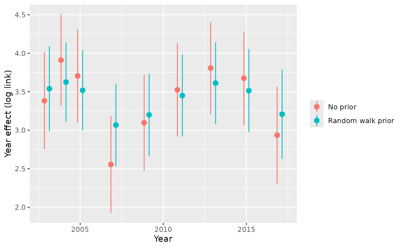

This example shows how far custom priors can go; most uses will be simpler.

A gamma prior on a time-varying SD

Instead of fixed year effects, we can let the intercept follow a random walk with time_varying = ~ 1. The SD of the random walk steps is theta$sigma_V (its raw parameter is par$ln_tau_V = log(sigma_V)). The rows are the time-varying coefficients (only the intercept here) and the columns are model components.

fit_tv <- sdmTMB(
  density ~ 0 + depth_scaled + depth_scaled2,
  data = pcod,
  mesh = mesh,
  family = tweedie(),
  time = "year",
  time_varying = ~ 1,
  time_varying_type = "rw0",
  spatiotemporal = "off",
  extra_time = min(pcod$year):max(pcod$year)
)
get_prior_parameters(fit_tv) |> subset(name %in% c("ln_tau_V", "sigma_V"))
#>             expression  list     name label     value    status
#> 8   par$ln_tau_V[1, 1]   par ln_tau_V  <NA> 0.2091255 estimated
#> 18 theta$sigma_V[1, 1] theta  sigma_V  <NA> 1.2325996   derived

A gamma prior is often easier to specify through its mean and coefficient of variation (CV) than its shape and scale. A gamma with mean mu and CV cv has shape = 1 / cv^2 and scale = cv^2 * mu. Here’s a prior with a mean of 0.2 and a CV of 0.3 on the SD of the year-to-year changes in the intercept:

mu <- 0.2
cv <- 0.3
fit_tv_gamma <- update(fit_tv, priors = sdmTMBpriors(
  custom = function(par, theta) {
    c(sigma_V = RTMB::dgamma(theta$sigma_V[1, 1],
      shape = 1 / cv^2, scale = cv^2 * mu, log = TRUE))
  }
))
get_prior_parameters(fit_tv) |> subset(name == "sigma_V")
#>             expression  list    name label  value  status
#> 18 theta$sigma_V[1, 1] theta sigma_V  <NA> 1.2326 derived
get_prior_parameters(fit_tv_gamma) |> subset(name == "sigma_V")
#>             expression  list    name label     value  status
#> 18 theta$sigma_V[1, 1] theta sigma_V  <NA> 0.3138175 derived

This prior is also available built in as sdmTMBpriors(sigma_V = gamma_cv(mu, cv)), which gives the same fit. The custom version is a starting point for other distributions or for linking priors across coefficients. For a Bayesian fit, the log Jacobian from ln_tau_V to sigma_V is par$ln_tau_V[1, 1]. We’ll talk more about that next.

Penalties versus Bayesian priors and Jacobians

When fitting by maximum likelihood (the default), a custom prior is a penalty on the likelihood, and the optimum is the posterior mode on the scale the prior is written on. No Jacobian is needed. For a Bayesian fit (see the Bayesian vignette), a prior on a transformed parameter needs a Jacobian adjustment, because the sampler works with the raw parameters.

sdmTMB doesn’t automatically work out the Jacobian for a custom prior for you. Instead, supply its log in custom_log_jacobian, which is only used with bayesian = TRUE. For the normal prior on the log range, the raw parameter is ln_kappa and log(range) = log(sqrt(8)) - ln_kappa. The absolute derivative of log(range) with respect to ln_kappa is 1, so the log Jacobian is 0 and no adjustment is needed. For the half-normal prior on phi = exp(ln_phi), the log Jacobian is ln_phi:

fit_bayes <- update(fit,
  bayesian = TRUE,
  priors = sdmTMBpriors(
    custom = function(par, theta) {
      RTMB::dnorm(theta$phi[1], 0, 20, log = TRUE)
    },
    custom_log_jacobian = function(par, theta) {
      par$ln_phi[1]
    }
  )
)

A prior directly on a raw parameter as it enters the model, such as par$ln_phi, never needs a Jacobian.

The Matérn range and field standard deviations

The Matérn range and the field standard deviations (sigma_O, sigma_E) are more complex than most parameters because they depend on each other. The range depends only on ln_kappa, but each standard deviation depends on both ln_kappa and its ln_tau_*. So the Jacobian for a prior on sigma_E alone isn’t well defined: it has to come from the joint transformation from (ln_kappa, ln_tau_E) to (range, sigma_E). The log Jacobian of that transformation is log(range) + log(sigma_E). With a shared range (the default, share_range = TRUE), one ln_kappa maps to the range for both fields, so add log(range) once plus log(sigma) for each field.

For example, for a Bayesian fit with the range and sigma_E priors from earlier, the prior on log(range) and sigma_E together needs a log Jacobian of log(sigma_E). The log(range) term from the joint transformation cancels with the -log(range) from putting the prior on log(range) rather than range:

fit_bayes_range <- update(fit,
  bayesian = TRUE,
  priors = sdmTMBpriors(
    custom = function(par, theta) {
      c(
        range = RTMB::dnorm(log(theta$range[1, 1]), log(50), 0.3, log = TRUE),
        sigma_E = RTMB::dnorm(theta$sigma_E[1, 1], 0, 0.5, log = TRUE)
      )
    },
    custom_log_jacobian = function(par, theta) {
      theta$log_sigma_E[1, 1]
    }
  )
)

This model also has a spatial field, which shares the range. Without a custom prior on sigma_O, its ln_tau_O keeps a flat prior on its raw scale.

For priors on these parameters, we suggest the built-in penalized complexity (PC) priors instead: pc_matern() through the matern_s and matern_st arguments to sdmTMBpriors(). They put a joint prior on the range and standard deviation of each field and take care of the Jacobian for you when bayesian = TRUE.

Limitations

• Custom priors need the RTMB backend.
• Like the built-in priors, custom priors are part of the model’s objective, so they’re included in logLik() and AIC().
• The names and shapes of par and theta are internal and could change in future versions. Check them with get_prior_parameters().