Forecasting with sdmTMB

Here we will cover using sdmTMB for forecasting data in time or extrapolating spatially to unsampled areas. These forecasting approaches have multiple applications, including:

predicting for future years
interpolating over missed years
extrapolating in space to unsampled areas (e.g., an area beyond the existing domain)
interpolating in space within the existing spatial domain

Forecasting: predicting for future time and interpolating over missed time slices

Predicting for future time and interpolating over missed time requires a similar method, so we will cover them both here. To forecast in time, either future or missed time, we need a model for time. For example, a model with year as a factor (e.g., 0 + as.factor(year)) can’t predict for years without data, because no coefficient is estimated for those years.

The options for including time in the model include:

AR(1) or random walk spatiotemporal fields
Random walk intercepts
Smoothers on the time variable (e.g., s(year))
Ignoring time (e.g., a spatial-only model, so predictions are identical across years)
Some combination of these

We will use the Pacific cod data to show how to implement each of these options.

First, we need to make our mesh.

mesh <- make_mesh(pcod, c("X", "Y"), cutoff = 20)

Next, we need to create a vector of the years that we want the model to include. The DFO survey in this region only includes years 2003, 2004, 2005, 2007, 2009, 2011, 2013, 2015, and 2017. To fill in Pacific cod density for the unsampled years and forecast into the future, we can simply give the model every year we want, from the first survey year through the last forecast year (here, 2025). Years that are already in the data are fine to include.

all_years <- 2003:2025

Then, we will fit a model of Pacific cod density that includes a quadratic effect of depth. The argument extra_time in the sdmTMB() function is how we will add in interpolation and forecasting. We also will need to set the argument time to time = "year".

In this example, we will choose to turn off spatial random fields (spatial = "off"), so we are only including spatiotemporal random fields.

We then have different options for including time in the model.

AR(1) spatiotemporal field

To include spatiotemporal variation as an AR(1) process, we can specify spatiotemporal = "AR1":

fit_ar1 <- sdmTMB(
  density ~ depth_scaled + depth_scaled2,
  time = "year",
  extra_time = all_years, #<< all years to include, with or without data
  spatiotemporal = "AR1", #<< setting an AR(1) spatiotemporal process
  data = pcod,
  mesh = mesh,
  family = tweedie(link = "log"),
  spatial = "off",
  silent = FALSE #< monitor progress
)

Random walk spatiotemporal field

Or, we can set spatiotemporal variation to a random walk with spatiotemporal = "RW":

fit_rw <- sdmTMB(
  density ~ depth_scaled + depth_scaled2,
  time = "year",
  extra_time = all_years, #<<
  spatiotemporal = "RW", #<<
  data = pcod,
  mesh = mesh,
  family = tweedie(link = "log"),
  spatial = "off",
  silent = FALSE
)

Random walk intercept + AR(1) fields

We can also model the intercept as a random walk by removing the intercept from the main formula (adding 0 to the formula) and including the argument time_varying = ~1:

fit_rw_ar1 <- sdmTMB(
  density ~ 0 + depth_scaled + depth_scaled2, #<< remove intercept with 0
  time = "year",
  time_varying = ~1, #<< instead include the intercept here as a random walk
  extra_time = all_years,
  spatiotemporal = "AR1", #<<
  data = pcod,
  mesh = mesh,
  family = tweedie(link = "log"),
  spatial = "off",
  silent = FALSE
)

Smoother on year + AR(1) fields

We can also add a smoother on year with s(year) in the formula while keeping spatiotemporal = "AR1":

fit_sm <- sdmTMB(
  density ~ s(year, k = 5) + depth_scaled + depth_scaled2, #<< add smoother on year
  time = "year",
  extra_time = all_years, #<<
  spatiotemporal = "AR1", #<<
  data = pcod,
  mesh = mesh,
  family = tweedie(link = "log"),
  spatial = "off",
  silent = FALSE
)

Deciding between methods

In deciding which method (AR(1), RW, etc.) to use for including time in the model, it is important to know that:

AR(1) field processes revert towards the mean
Random walk processes (in the mean or time-varying parameters) do not revert towards the mean
Smoothers should be used with caution for forecasting: beyond the data they extrapolate the shape of the basis functions, which can produce unrealistic trends
Uncertainties in prediction for random walks, AR(1) processes, and smoothers increase the further away we get from data

`project()` function for faster long-term forecasting

Because forecasting with extra_time can be slow—especially for large datasets or for projections far into the future—sdmTMB also includes a project() function for doing projections via simulation. Instead of estimating the future random fields as part of the fit, project() fits the model to the historical years only and then simulates the future random fields. This is based on an approach first developed in the project_model() function in VAST.

Using the built-in dogfish dataset, we’ll first define the years for the historical (fitting) and projection periods.

mesh <- make_mesh(dogfish, c("X", "Y"), cutoff = 30)
historical_years <- 2004:2022
to_project <- 5
future_years <- seq(max(historical_years) + 1, max(historical_years) + to_project)
all_years <- c(historical_years, future_years)
proj_grid <- replicate_df(wcvi_grid, "year", all_years)

Next, we’ll fit the model. We’ll use an AR(1) spatiotemporal field, which drives the future forecasts.

fit <- sdmTMB(
  catch_weight ~ 1,
  time = "year",
  offset = log(dogfish$area_swept),
  extra_time = historical_years, #< fills in historical years without data; does *not* include projection years
  spatial = "on",
  spatiotemporal = "AR1",
  data = dogfish,
  mesh = mesh,
  family = tweedie(link = "log")
)

Finally, we’ll do the projections. We’ll only use 20 draws for speed and simplicity, but you should increase this for real-world applications so that you have stable results.

set.seed(1)
out <- project(fit, newdata = proj_grid, nsim = 20)

out is a list with elements est and epsilon_st, each a matrix with one row per row of proj_grid and one column per draw (here, 20). The first (est) contains the predictions and the second (epsilon_st) contains the spatiotemporal random effects, both in link (here, log) space. These can be summarized and visualized in several ways to show trends in both the mean and uncertainty intervals (e.g., quantiles across draws).

For example, here is the mean of the projections:

proj_grid$est_mean <- apply(out$est, 1, mean)
ggplot(subset(proj_grid, year %in% future_years), aes(X, Y, fill = est_mean)) +
  geom_raster() +
  facet_wrap(~year) +
  coord_fixed() +
  scale_fill_viridis_c() +
  labs(fill = "Mean\n(log space)")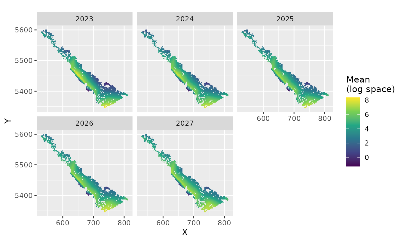

By default, project() samples estimated parameter uncertainty and the historical latent states, then simulates future spatiotemporal and time-varying effects. If you want to keep those uncertainty sources but propagate future random effects at their conditional means (i.e., exclude future process uncertainty), use sample_future_re = FALSE. Comparing the two shows how much of the projection uncertainty comes from future process variability:

out_mean_future <- project(
  fit, newdata = proj_grid, nsim = 20, sample_future_re = FALSE
)
#> Fitted object contains an offset but the offset is `NULL` in `predict.sdmTMB()`
#> and `newdata` were supplied.
#> Prediction will proceed assuming the offset vector is 0 in the prediction.
#> Specify an offset vector in `predict.sdmTMB()` to override this.
#> Rebuilding TMB object with TMB::MakeADFun()
proj_grid$sd_full <- apply(out$est, 1, sd)
proj_grid$sd_mean_future <- apply(out_mean_future$est, 1, sd)
proj_grid |>
  dplyr::group_by(year) |>
  dplyr::summarise(
    sd_full = mean(sd_full),
    sd_mean_future = mean(sd_mean_future)
  ) |>
  dplyr::filter(year %in% future_years)
#> # A tibble: 5 × 3
#>    year sd_full sd_mean_future
#>   <int>   <dbl>          <dbl>
#> 1  2023    1.41          0.702
#> 2  2024    1.65          0.740
#> 3  2025    1.75          0.788
#> 4  2026    1.82          0.830
#> 5  2027    1.86          0.865

See the help file ?sdmTMB::project for additional examples.

Interpolating in space to unsampled areas

We can also interpolate predicted values to unsampled areas within the geographic extent of the data. For this example, we will use the data on the locations of 3605 trees in a 1000 by 500 m rectangular sampling region from the spatstat.data package.

First we will create a data frame of the x and y coordinates from the tree dataset, and we can map the locations:

dat <- data.frame(
  x = spatstat.data::bei$x,
  y = spatstat.data::bei$y
)
ggplot(dat, aes(x, y)) +
  geom_point(col = "darkblue", alpha = 0.1) +
  coord_cartesian(expand = FALSE)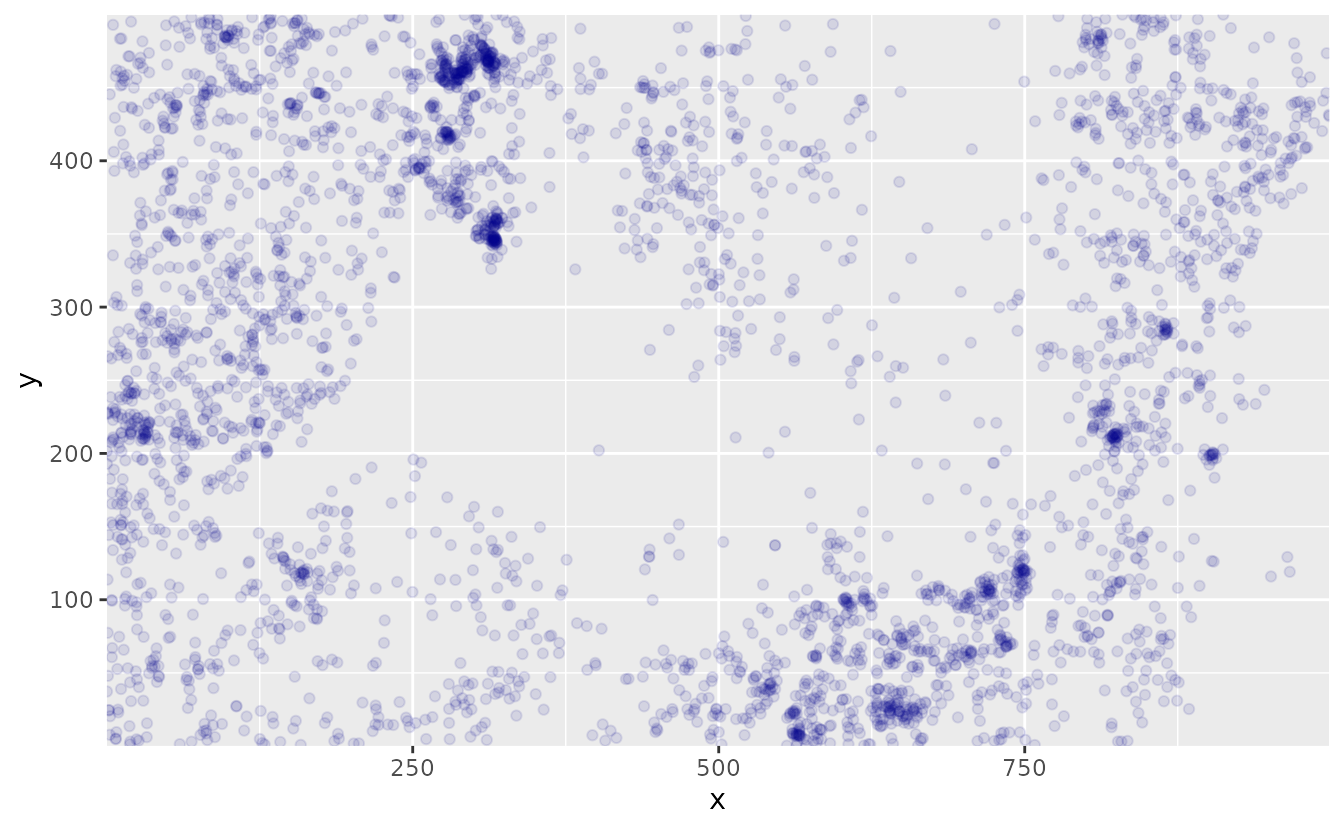

Next, we re-format the data to create density observations. We bin the tree locations into 50 × 50 m cells and count the number of trees in each cell. A larger cell size gives a coarser resolution. Then, we create the mesh and visualize it.

cell_size <- 50 # controls resolution
dat$x <- cell_size * floor(dat$x / cell_size)
dat$y <- cell_size * floor(dat$y / cell_size)

dat <- dplyr::group_by(dat, x, y) |>
  dplyr::summarise(n = n())

mesh <- make_mesh(
  dat,
  xy_cols = c("x", "y"),
  cutoff = 80 # min. distance between knots in X-Y units
)
plot(mesh)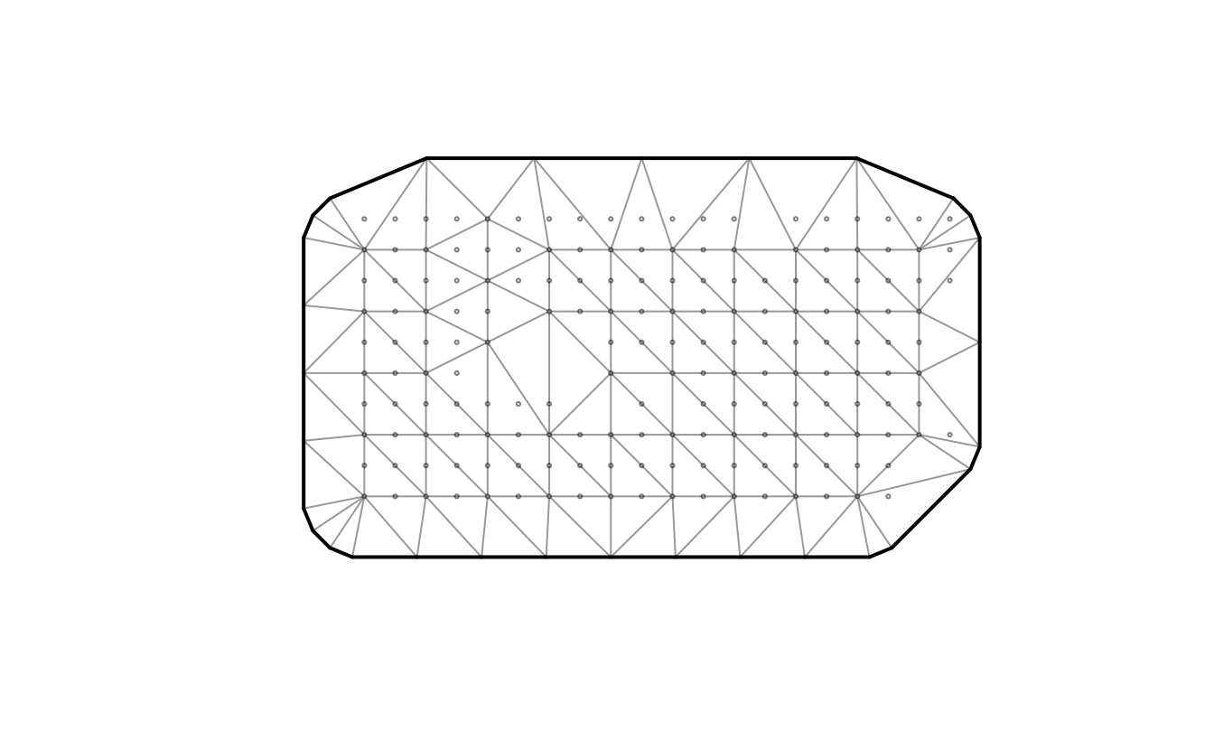

Then, we can fit a model of tree density with only an intercept and a single time slice. Because we only kept cells that contain at least one tree, there are no zeros in the data, so we use a zero-truncated negative binomial family (truncated_nbinom2()).

fit <- sdmTMB(n ~ 1,
  data = dat,
  mesh = mesh,
  family = truncated_nbinom2(link = "log")
)

Next, we can predict to unsampled areas within the geographic extent of our data. We first expand the grid by adding in x and y coordinates between existing coordinates in our dataset. Here, we will add in points at intervals of 5 for x and y. This value controls the resolution of predicted data. Increasing the value will decrease the resolution of spatial predictions.

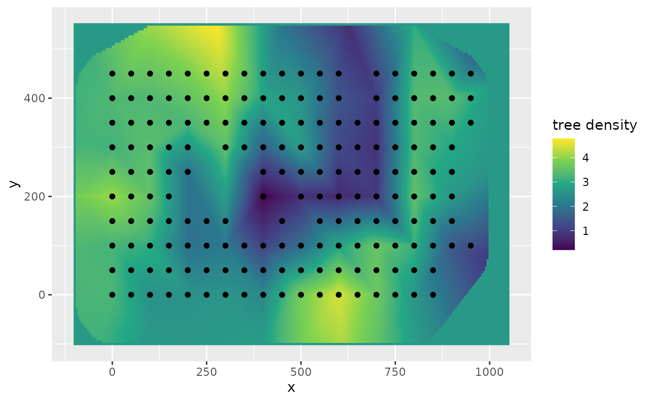
We can map the predicted tree density at each of our interpolated points compared to the locations of our data to see the increased resolution from interpolating with this method. Note that predictions are in link (log) space.

# makes all combinations of x and y:
newdf <- expand.grid(
  x = seq(min(dat$x), max(dat$x), 5),
  y = seq(min(dat$y), max(dat$y), 5)
)
p <- predict(fit, newdata = newdf)

ggplot(p, aes(x, y)) +
  geom_raster(data = p, aes(x, y, fill = est)) +
  geom_point(data = dat, aes(x, y)) +
  labs(fill = "log tree density") +
  scale_fill_viridis_c()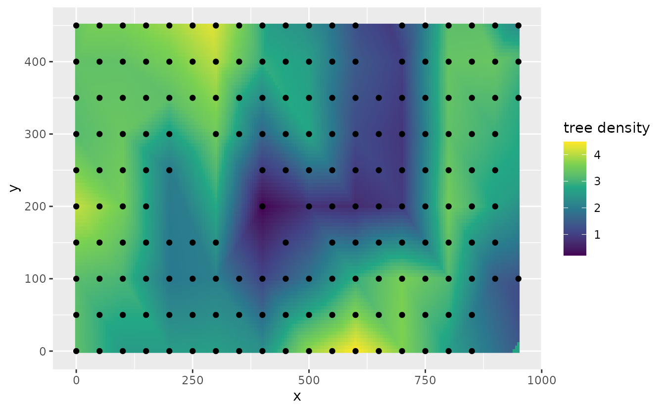

We can also add the argument nsim = 200 when predicting, which returns a matrix of 200 draws (columns) for each prediction location (rows) in link space, and then summarize the draws. Here, we take the mean:

p2 <- predict(fit, newdata = newdf, nsim = 200)
newdf$p2 <- apply(p2, 1, mean)
ggplot(newdf, aes(x, y)) +
  geom_raster(data = newdf, aes(x, y, fill = p2)) +
  geom_point(data = dat, aes(x, y)) +
  labs(fill = "log tree density") +
  scale_fill_viridis_c()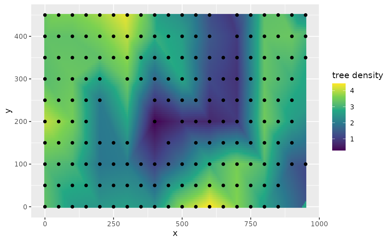

We can also visualize uncertainty in the interpolated predictions by mapping the standard deviation of the draws at each point in space. Uncertainty is higher near the edges of the domain and away from observations, where there is less information to inform the spatial field (see, e.g., this tutorial).

newdf$est_se <- apply(p2, 1, sd)
ggplot() +
  geom_raster(data = newdf, aes(x = x, y = y, fill = est_se)) +
  coord_equal() +
  labs(fill = "SD of prediction\n(log space)") +
  scale_fill_viridis_c(option = "D")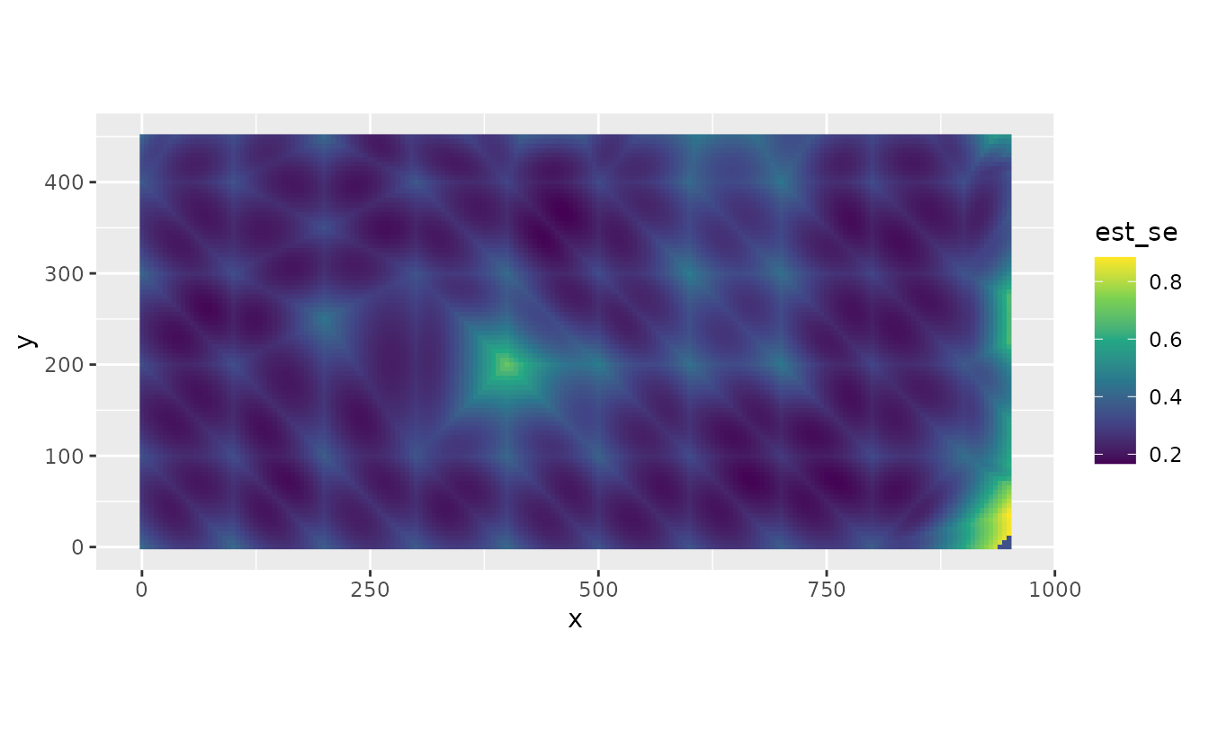

Extrapolating outside the sampled domain

We can also extrapolate spatially outside the geographic extent of the data. For instance, we can predict into a border area. To do so, we expand the x and y coordinates to values above and below the extent of the coordinates in the data. Here, we expand the geographic domain by 100 m in all directions and keep the resolution at 5 m. Then, we can use the same model fit to predict to the expanded geographic domain.

Be cautious when extrapolating: as we move away from the data, the spatial field reverts towards its mean of zero, so predictions approach the fixed effects alone. Beyond the mesh boundary, the spatial field is zero.

newdf <- expand.grid(
  x = seq(min(dat$x) - 100, max(dat$x) + 100, 5),
  y = seq(min(dat$y) - 100, max(dat$y) + 100, 5)
)
p3 <- predict(fit, newdata = newdf)
ggplot(p3, aes(x, y)) +
  geom_raster(data = p3, aes(x, y, fill = est)) +
  geom_point(data = dat, aes(x, y)) +
  labs(fill = "log tree density") +
  scale_fill_viridis_c()

Julia Indivero, Sean Anderson, Lewis Barnett, Philina English, Eric Ward, Jim Thorson

2026-10-15

Forecasting: predicting for future time and interpolating over missed time slices

AR(1) spatiotemporal field

Random walk spatiotemporal field

Random walk intercept + AR(1) fields

Smoother on year + AR(1) fields

Deciding between methods

`project()` function for faster long-term forecasting

Interpolating in space to unsampled areas

Extrapolating outside the sampled domain

Forecasting with sdmTMB

Julia Indivero, Sean Anderson, Lewis Barnett, Philina English, Eric Ward, Jim Thorson

2026-10-15

Forecasting: predicting for future time and interpolating over missed time slices

AR(1) spatiotemporal field

Random walk spatiotemporal field

Random walk intercept + AR(1) fields

Smoother on year + AR(1) fields

Deciding between methods

project() function for faster long-term forecasting

Interpolating in space to unsampled areas

Extrapolating outside the sampled domain

`project()` function for faster long-term forecasting