Project from an sdmTMB model using simulation

Project forward in time from an sdmTMB model using a simulation approach for computational efficiency. This can be helpful for calculating predictive intervals for long projections where including those time elements in extra_time during model estimation can be slow.

Inspiration for this approach comes from the VAST function project_model().

Usage

project(
  object,
  newdata,
  nsim = 1,
  sample_fe = TRUE,
  sample_historical_re = TRUE,
  sample_future_re = TRUE,
  future_re = c("include", "zero", "fix"),
  silent = FALSE,
  sims_var = NULL,
  return_tmb_report = FALSE,
  ...
)

Arguments

object: A fitted model from sdmTMB().
newdata: A new data frame to predict on. It should contain both the historical time elements and any new time elements to project to. Time values must be numeric and align with the constant cadence in the fitted model. Missing intermediate future time elements are simulated.
nsim: Number of projection simulations.
sample_fe: Logical. Sample uncertainty in the estimated model parameters, including regression coefficients, covariance parameters, and dispersion parameters.
sample_historical_re: Logical. Sample uncertainty in random effects associated with the fitted historical period.
sample_future_re: Logical. Simulate random effects in the projection period. When FALSE, dynamic effects are propagated at their conditional means. Ignored when future_re is "zero" or "fix".
future_re: Treatment of spatiotemporal random effects and time-varying coefficients in the projection period. "include" preserves the usual process dynamics, "zero" sets them to zero, and "fix" holds them at their value in the final historical time step. Historical effects are unchanged.
silent: Logical. Suppress progress messages?
sims_var: Optional single element to extract from the TMB simulation report. If NULL, the default, the usual named projection list is returned. If supplied, use a native projection report name such as "proj_eta" or "proj_epsilon_st_A_vec"; the simulation dimension is last. See also return_tmb_report.
return_tmb_report: Return the TMB report from simulate()? This lets you parse out whatever elements you want from the simulation including grabbing multiple elements from one set of simulations. Prediction-path elements retain their native proj_* names. See examples.
...: Passed to predict.sdmTMB().

Value

Default: a list with elements est and epsilon_st (if spatiotemporal effects are present). Each list element includes a matrix with rows corresponding to rows in newdata and nsim columns. For delta models, the components are est1, est2, epsilon_st, and epsilon_st2 for the 1st and 2nd linear predictors. In all cases, these returned values are in link space.

If sims_var is supplied, an array containing that report element, with the simulation dimension last. If return_tmb_report = TRUE, a list of TMB reports returned by simulate(). Run names() on an element of the output to see the available sims_var options. Unprefixed observation-path reports such as eta_i describe the historical fitting data; projected newdata values are in the corresponding proj_* reports.

References

project_model() in the VAST package.

Author

J.T. Thorson wrote the original version in the VAST package. S.C. Anderson wrote this version inspired by the VAST version with help from A.J. Allyn.

Examples

# \donttest{
if (ggplot2_installed()) {
library(ggplot2)

mesh <- make_mesh(dogfish, c("X", "Y"), cutoff = 25)
historical_years <- 2004:2022
to_project <- 10
future_years <- seq(max(historical_years) + 1, max(historical_years) + to_project)
all_years <- c(historical_years, future_years)
proj_grid <- replicate_df(wcvi_grid, "year", all_years)

# we could fit our model like this, but for long projections, this becomes slow:
if (FALSE) {
  fit <- sdmTMB(
    catch_weight ~ 1,
    time = "year",
    offset = log(dogfish$area_swept),
    extra_time = all_years, #< note that all years here
    spatial = "on",
    spatiotemporal = "ar1",
    data = dogfish,
    mesh = mesh,
    family = tweedie(link = "log")
  )
}

# instead, we could fit our model like this and then take simulation draws
# from the projection time period:
fit2 <- sdmTMB(
  catch_weight ~ 1,
  time = "year",
  offset = log(dogfish$area_swept),
  extra_time = historical_years, #< does *not* include projection years
  spatial = "on",
  spatiotemporal = "ar1",
  data = dogfish,
  mesh = mesh,
  family = tweedie(link = "log")
)

# we will only use 20 `nsim` so this example runs quickly
# you will likely want many more (> 200) in practice so the result
# is relatively stable

set.seed(1)
out <- project(fit2, newdata = proj_grid, nsim = 20)
names(out)
est_mean <- apply(out$est, 1, mean) # summarize however you'd like
est_se <- apply(out$est, 1, sd)

# Keep parameter and historical-state uncertainty, while propagating future
# dynamic effects at their conditional means:
out_mean_future <- project(
  fit2, newdata = proj_grid, nsim = 20, sample_future_re = FALSE
)

# visualize:
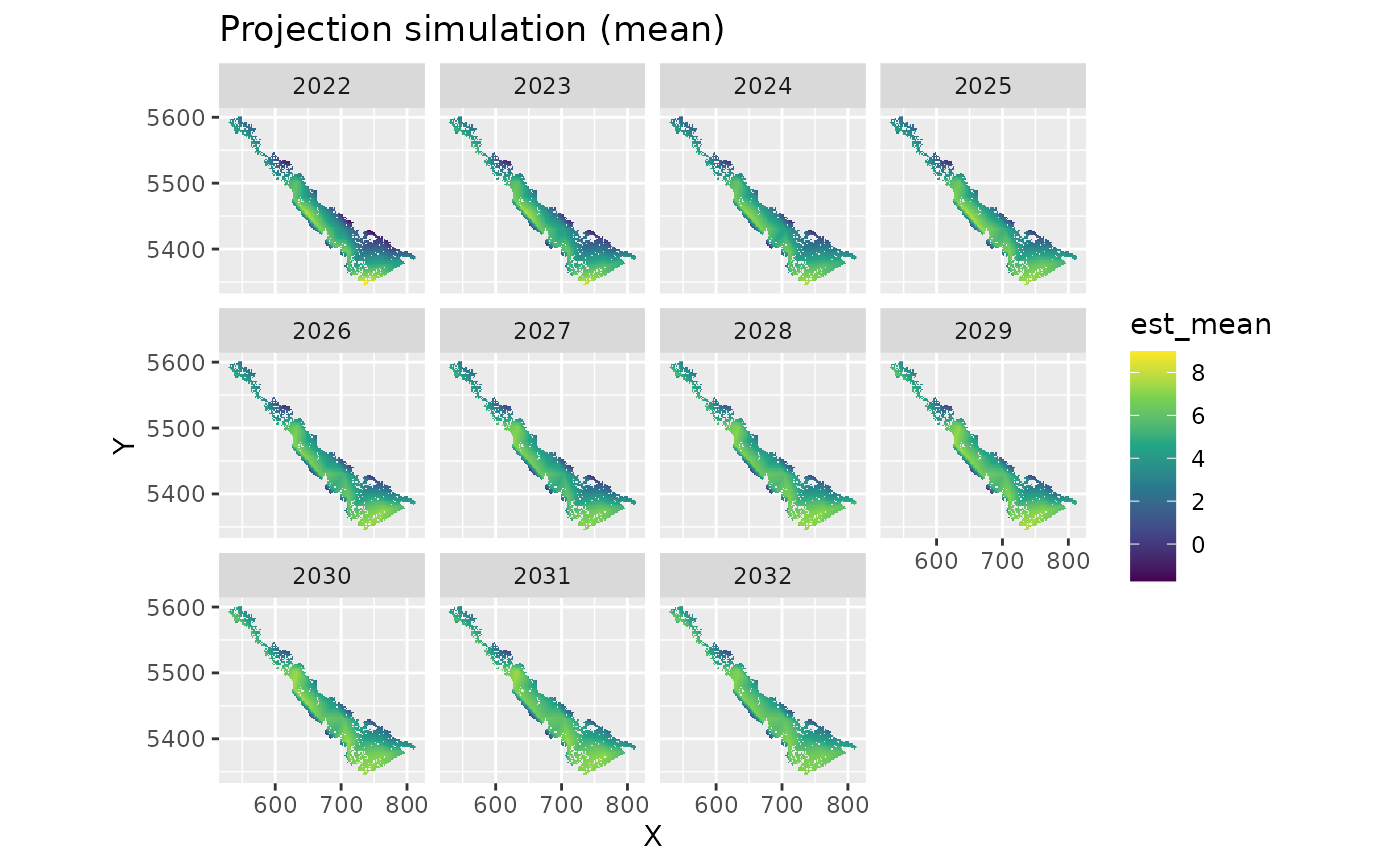
proj_grid$est_mean <- est_mean
ggplot(subset(proj_grid, year > 2021), aes(X, Y, fill = est_mean)) +
  geom_raster() +
  facet_wrap(~year) +
  coord_fixed() +
  scale_fill_viridis_c() +
  ggtitle("Projection simulation (mean)")

# visualize the spatiotemporal random fields:
proj_grid$eps_mean <- apply(out$epsilon_st, 1, mean)
proj_grid$eps_se <- apply(out$epsilon_st, 1, sd)
ggplot(subset(proj_grid, year > 2021), aes(X, Y, fill = eps_mean)) +
  geom_raster() +
  facet_wrap(~year) +
  scale_fill_gradient2() +
  coord_fixed() +
  ggtitle("Projection simulation\n(spatiotemporal fields)")

ggplot(subset(proj_grid, year > 2021), aes(X, Y, fill = eps_se)) +
  geom_raster() +
  facet_wrap(~year) +
  scale_fill_viridis_c() +
  coord_fixed() +
  ggtitle("Projection simulation\n(spatiotemporal fields standard error)")
}
#> Fitted object contains an offset but the offset is `NULL` in `predict.sdmTMB()`
#> and `newdata` were supplied.
#> Prediction will proceed assuming the offset vector is 0 in the prediction.
#> Specify an offset vector in `predict.sdmTMB()` to override this.
#> Rebuilding TMB object with TMB::MakeADFun()
#> Fitted object contains an offset but the offset is `NULL` in `predict.sdmTMB()`
#> and `newdata` were supplied.
#> Prediction will proceed assuming the offset vector is 0 in the prediction.
#> Specify an offset vector in `predict.sdmTMB()` to override this.
#> Rebuilding TMB object with TMB::MakeADFun()

# }