Index standardization with sdmTMB
2026-10-05
Source:vignettes/articles/index-standardization.Rmd
index-standardization.RmdIf the code in this vignette has not been evaluated, a rendered version is available on the documentation site under ‘Articles’.
Let’s perform index standardization with the built-in data for Pacific Cod.
- The density units should be kg/km2.
- Here, X and Y are coordinates in UTM zone 9.
glimpse(pcod)
#> Rows: 2,143
#> Columns: 12
#> $ year          <int> 2003, 2003, 2003, 2003, 2003, 2003, 2003, 2003, 2003, 20…
#> $ X             <dbl> 446.4752, 446.4594, 448.5987, 436.9157, 420.6101, 417.71…
#> $ Y             <dbl> 5793.426, 5800.136, 5801.687, 5802.305, 5771.055, 5772.2…
#> $ depth         <dbl> 201, 212, 220, 197, 256, 293, 410, 387, 285, 270, 381, 1…
#> $ density       <dbl> 113.138476, 41.704922, 0.000000, 15.706138, 0.000000, 0.…
#> $ present       <dbl> 1, 1, 0, 1, 0, 0, 0, 0, 0, 1, 0, 0, 0, 0, 0, 0, 0, 0, 0,…
#> $ lat           <dbl> 52.28858, 52.34890, 52.36305, 52.36738, 52.08437, 52.094…
#> $ lon           <dbl> -129.7847, -129.7860, -129.7549, -129.9265, -130.1586, -…
#> $ depth_mean    <dbl> 5.155194, 5.155194, 5.155194, 5.155194, 5.155194, 5.1551…
#> $ depth_sd      <dbl> 0.4448783, 0.4448783, 0.4448783, 0.4448783, 0.4448783, 0…
#> $ depth_scaled  <dbl> 0.3329252, 0.4526914, 0.5359529, 0.2877417, 0.8766077, 1…
#> $ depth_scaled2 <dbl> 0.11083919, 0.20492947, 0.28724555, 0.08279527, 0.768440…
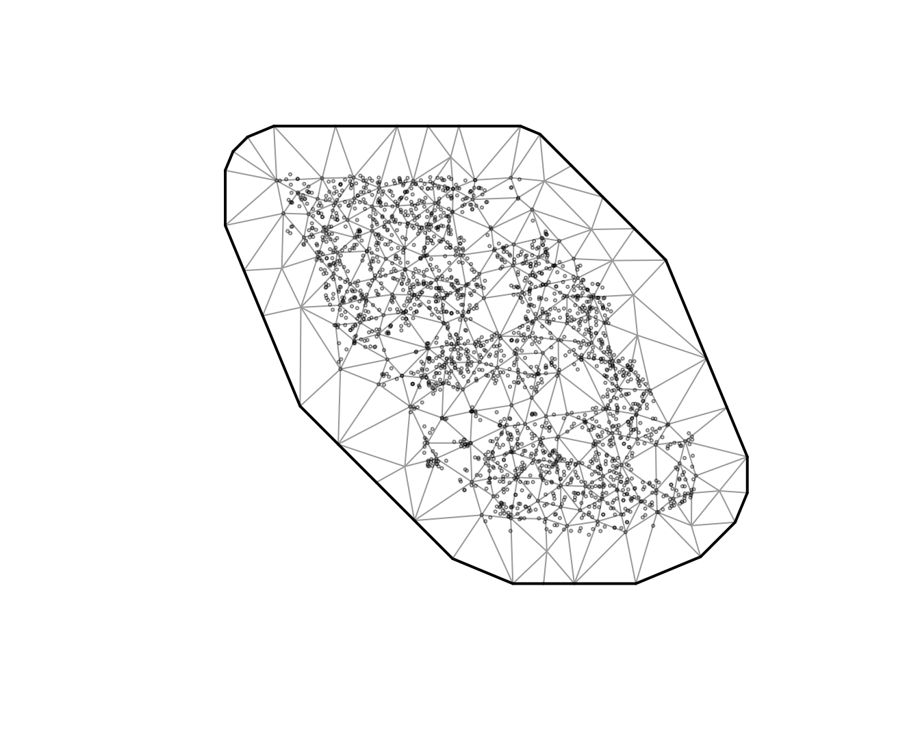
First we will create our SPDE mesh. We will use a relatively coarse
mesh as a balance between speed and accuracy in this vignette
(cutoff = 10, where cutoff is in the units of X and Y (km
here) and represents the minimum distance between points before a new
mesh vertex is added). In applied scenarios, you will likely want to use
a finer mesh and check that increasing the number of knots does not
change the conclusions.
Let’s fit a GLMM. Note that if you want to use this model for index
standardization, then you will likely want to include
0 + as.factor(year) or -1 + as.factor(year) so
that there is a factor predictor representing the mean estimate for each
time slice.
m <- sdmTMB(
  data = pcod,
  formula = density ~ 0 + as.factor(year),
  time = "year", mesh = pcod_spde, family = tweedie(link = "log"))
We can inspect randomized quantile residuals:
pcod$resids <- residuals(m) # randomized quantile residuals
# Also see residuals(..., type = "mle-mcmc") which are better but slower
hist(pcod$resids)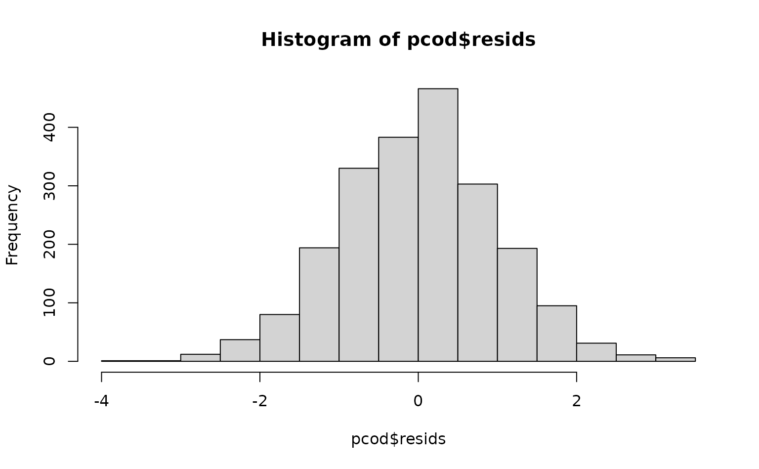

ggplot(pcod, aes(X, Y, col = resids)) + scale_colour_gradient2() +
  geom_point() + facet_wrap(~year) + coord_fixed()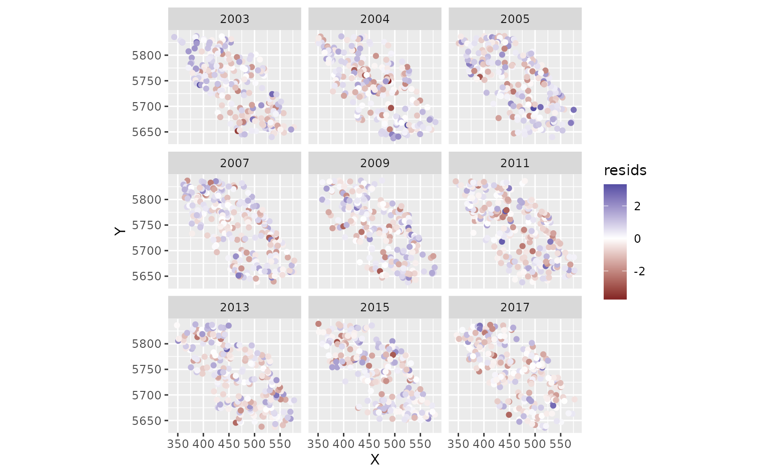
Now we want to predict on a fine-scale grid over the entire survey
domain. There is a grid built into the package for Queen Charlotte Sound
named qcs_grid. Our prediction grid also needs to have all
the covariates that we used in the model above.
glimpse(qcs_grid)
#> Rows: 7,314
#> Columns: 5
#> $ X             <dbl> 456, 458, 460, 462, 464, 466, 468, 470, 472, 474, 476, 4…
#> $ Y             <dbl> 5636, 5636, 5636, 5636, 5636, 5636, 5636, 5636, 5636, 56…
#> $ depth         <dbl> 347.08345, 223.33479, 203.74085, 183.29868, 182.99983, 1…
#> $ depth_scaled  <dbl> 1.56081222, 0.56976988, 0.36336929, 0.12570465, 0.122036…
#> $ depth_scaled2 <dbl> 2.436134794, 0.324637712, 0.132037240, 0.015801659, 0.01…
We can replicate our grid across all years:
grid_yrs <- replicate_df(qcs_grid, "year", unique(pcod$year))Now make predictions on the new data for mapping.
predictions <- predict(m, newdata = grid_yrs)Let’s make a small function to help make maps.
plot_map <- function(dat, column) {
  ggplot(dat, aes(X, Y, fill = {{ column }})) +
    geom_raster() +
    facet_wrap(~year) +
    coord_fixed()
}
There are four kinds of predictions that we get out of the model. First, we will show the predictions that incorporate all fixed and random effects:
plot_map(predictions, exp(est)) +
  scale_fill_viridis_c(trans = "sqrt") +
  ggtitle("Prediction (fixed effects + all random effects)")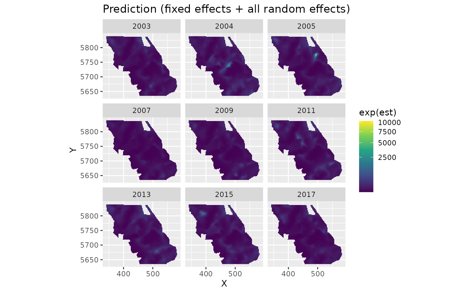
We can also look at just the fixed effects, here year:
plot_map(predictions, exp(est_non_rf)) +
  ggtitle("Prediction (fixed effects only)") +
  scale_fill_viridis_c(trans = "sqrt")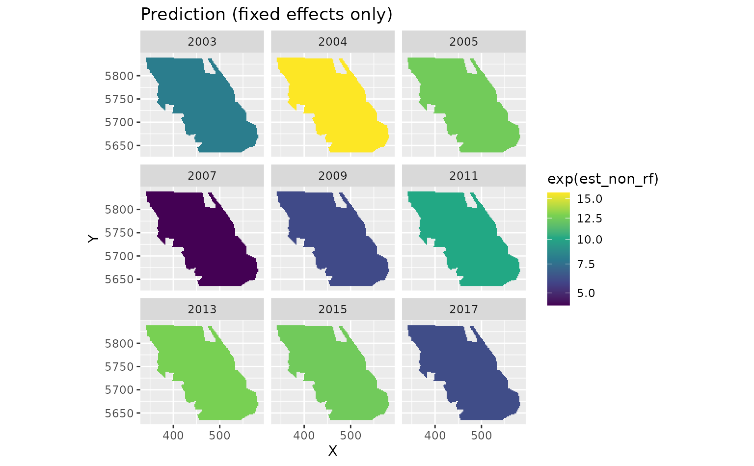
We can look at the spatial random effects that represent persistent deviations in space through time that are not accounted for by our fixed effects. In other words, these deviations represent persistent biotic and abiotic factors affecting biomass density that are not accounted for in the model.
plot_map(predictions, omega_s) +
  ggtitle("Spatial random effects only") +
  scale_fill_gradient2()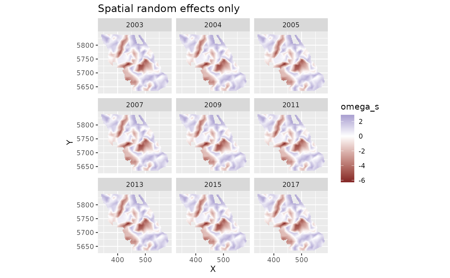
And finally we can look at the spatiotemporal random effects that represent deviations from the fixed-effect predictions and the spatial random-effect deviations. These represent biotic and abiotic factors that change through time and are not accounted for in the model.
plot_map(predictions, epsilon_st) +
  ggtitle("Spatiotemporal random effects only") +
  scale_fill_gradient2()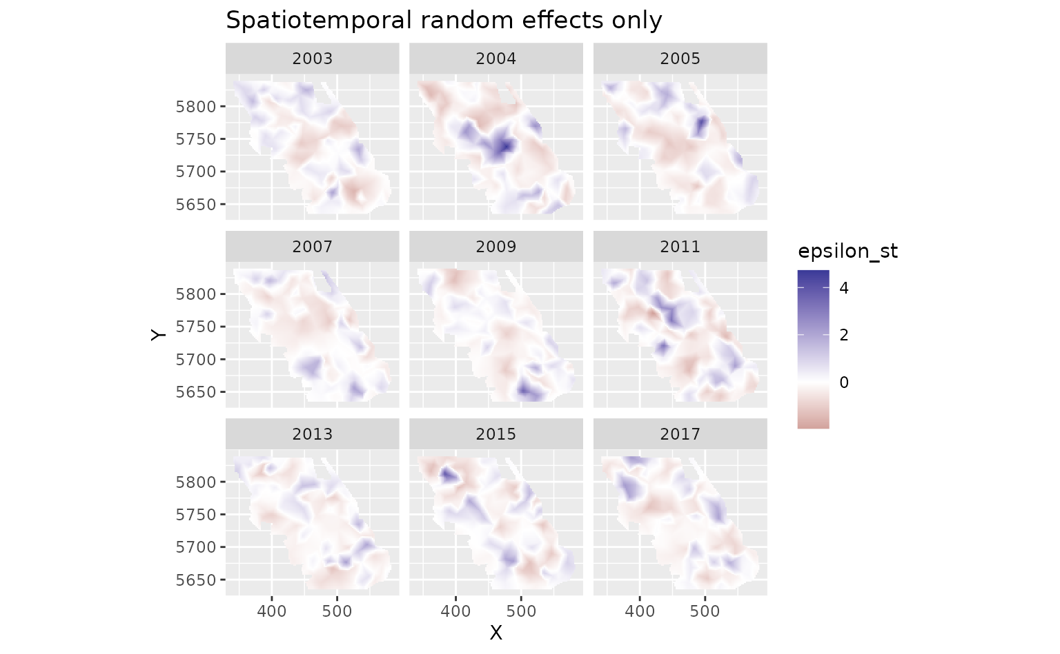
We can pass the fitted model and prediction grid directly to
get_index() to calculate total biomass estimates and
standard errors.
We will need to set the area argument to 4
km2 since our grid cells are 2 km x 2 km. If some grid cells
were not fully in the survey domain (or were on land), we could instead
pass a vector of grid-cell areas to the area argument
matching the number of grid cells.
index <- get_index(m, newdata = grid_yrs, area = 4, bias_correct = TRUE)
ggplot(index, aes(year, est)) + geom_line() +
  geom_ribbon(aes(ymin = lwr, ymax = upr), alpha = 0.4) +
  xlab('Year') + ylab('Biomass estimate (kg)')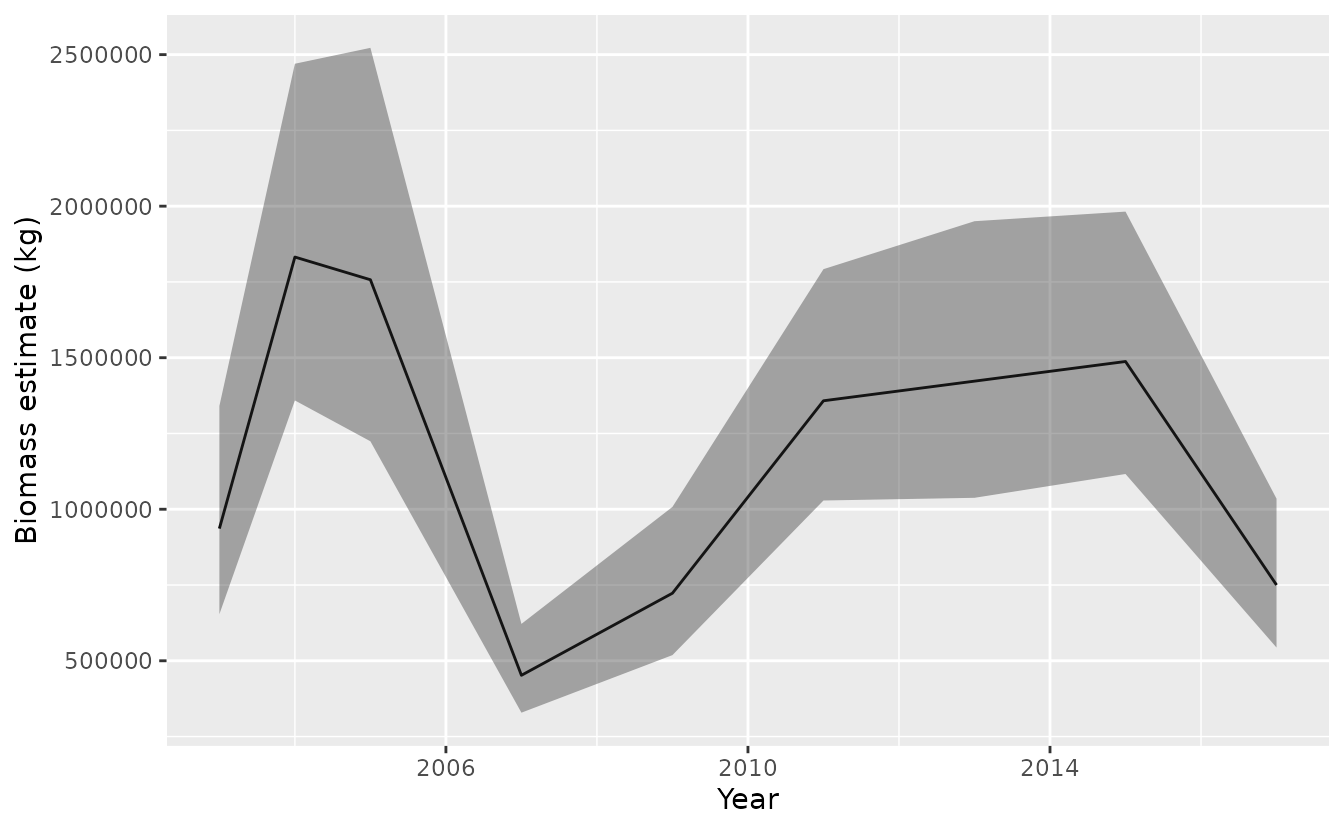
These are our biomass estimates:
mutate(index, cv = sqrt(exp(se^2) - 1)) |>
  select(-log_est, -se) |>
knitr::kable(format = "pandoc", digits = c(0, 0, 0, 0, 2))| year | est | lwr | upr | se_natural | type | cv |
|---|---|---|---|---|---|---|
| 2003 | 936176 | 653699 | 1340716 | 121052.57 | index | 0 |
| 2004 | 1832130 | 1359020 | 2469943 | 206077.83 | index | 0 |
| 2005 | 1757227 | 1224189 | 2522360 | 245584.74 | index | 0 |
| 2007 | 452112 | 328786 | 621698 | 51575.11 | index | 0 |
| 2009 | 722982 | 518713 | 1007692 | 84575.57 | index | 0 |
| 2011 | 1357885 | 1028851 | 1792147 | 140481.41 | index | 0 |
| 2013 | 1422648 | 1037721 | 1950358 | 163466.86 | index | 0 |
| 2015 | 1487473 | 1116301 | 1982062 | 157251.14 | index | 0 |
| 2017 | 750051 | 543622 | 1034867 | 86863.62 | index | 0 |
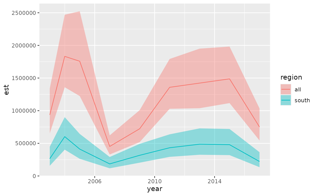
We can also calculate an index for part of the survey domain. We’ll
make an index for everything south of UTM 5700 by subsetting our
prediction grid. For more complicated spatial polygons, you could
intersect the polygon with the prediction grid using something like
sf::st_intersects().
qcs_grid_south <- grid_yrs[grid_yrs$Y < 5700, ]
index_south <- get_index(m, newdata = qcs_grid_south,
  area = 4, bias_correct = TRUE)
head(index_south)
#>   year      est      lwr      upr  log_est        se se_natural  type
#> 1 2003 264679.9 156368.9 448013.9 12.48628 0.2685270   49875.83 index
#> 2 2004 602466.8 403037.0 900577.8 13.30879 0.2051079   89491.31 index
#> 3 2005 411739.0 263138.9 644256.8 12.92814 0.2284265   66031.11 index
#> 4 2007 184945.7 117598.4 290861.9 12.12782 0.2310178   30159.18 index
#> 5 2009 316483.8 203600.9 491952.5 12.66503 0.2250603   50957.73 index
#> 6 2011 432243.6 292909.8 637857.0 12.97674 0.1985366   65227.12 index
We can visually compare the two indices:
mutate(index, region = "all") |>
  bind_rows(mutate(index_south, region = "south")) |>
  ggplot(aes(year, est)) +
  geom_line(aes(colour = region)) +
  geom_ribbon(aes(ymin = lwr, ymax = upr, fill = region), alpha = 0.4)