Residual checking with sdmTMB

If the code in this vignette has not been evaluated, a rendered version is available on the documentation site under ‘Articles’.

Residual checking with worked examples

library(sdmTMB)

We will start with some data simulated from scratch. We will simulate from an NB2 negative binomial observation model with a spatial random field, an intercept, and one predictor named a1 that has a linear effect on the observed data.

set.seed(1)
predictor_dat <- data.frame(X = runif(1000), Y = runif(1000), a1 = rnorm(1000))
mesh <- make_mesh(predictor_dat, xy_cols = c("X", "Y"), cutoff = 0.1)
dat <- sdmTMB_simulate(
  formula = ~ 1 + a1,
  data = predictor_dat,
  mesh = mesh,
  family = nbinom2(link = "log"),
  phi = 0.4,
  range = 0.4,
  sigma_O = 0.4,
  seed = 1,
  B = c(0.2, 0.8) # B0 = intercept, B1 = a1 slope
)

Next, we will fit model configurations with various families and predictors. The first model will use the Poisson instead of the NB2. The second model will match the simulated data. The third model is missing the ‘a1’ predictor. We’ll use a penalized complexity (PC) prior on the Matérn parameters to aid in estimation.

pc <- pc_matern(range_gt = 0.1, sigma_lt = 1)

fit_pois <- sdmTMB(observed ~ 1 + a1, data = dat, family = poisson(), mesh = mesh,
  priors = sdmTMBpriors(matern_s = pc))
fit_pois
#> Spatial model fit by ML ['sdmTMB']
#> Formula: observed ~ 1 + a1
#> Mesh: mesh (isotropic covariance)
#> Data: dat
#> Family: poisson(link = 'log')
#>  
#> Conditional model:
#>             coef.est coef.se
#> (Intercept)     0.27    0.17
#> a1              0.82    0.02
#> 
#> Matérn range: 0.12
#> Spatial SD: 1.20
#> ML criterion at convergence: 2887.957
#> 
#> See ?tidy.sdmTMB to extract these values as a data frame.

fit_nb2 <- update(fit_pois, family = nbinom2())
fit_nb2
#> Spatial model fit by ML ['sdmTMB']
#> Formula: observed ~ 1 + a1
#> Mesh: sdmTMBmesh (isotropic covariance)
#> Data: data.frame
#> Family: nbinom2(link = 'log')
#>  
#> Conditional model:
#>             coef.est coef.se
#> (Intercept)     0.52    0.14
#> a1              0.75    0.06
#> 
#> Dispersion parameter: 0.41
#> Matérn range: 0.29
#> Spatial SD: 0.42
#> ML criterion at convergence: 1735.452
#> 
#> See ?tidy.sdmTMB to extract these values as a data frame.

fit_nb2_miss <- update(fit_nb2, formula. = observed ~ 1)
fit_nb2_miss
#> Spatial model fit by ML ['sdmTMB']
#> Formula: observed ~ 1
#> Mesh: sdmTMBmesh (isotropic covariance)
#> Data: data.frame
#> Family: nbinom2(link = 'log')
#>  
#> Conditional model:
#>             coef.est coef.se
#> (Intercept)     0.77    0.14
#> 
#> Dispersion parameter: 0.30
#> Matérn range: 0.21
#> Spatial SD: 0.56
#> ML criterion at convergence: 1817.332
#> 
#> See ?tidy.sdmTMB to extract these values as a data frame.

We can see just by looking at these fits that the Poisson model inflates the spatial random-field standard deviation (SD) relative to the truth. The model missing the a1 predictor does so to a lesser degree.

Analytical randomized-quantile residuals

Here are randomized quantile residuals with fixed effects fixed at their MLEs (maximum likelihood estimates) and random effects taken from a single sample of their approximate distribution (more details below):

set.seed(123)
rq_res <- residuals(fit_pois, type = "mle-mvn")
rq_res <- rq_res[is.finite(rq_res)] # some Inf
qqnorm(rq_res);abline(0, 1)

set.seed(123)
rq_res <- residuals(fit_nb2, type = "mle-mvn")
qqnorm(rq_res);abline(0, 1)

These use the randomized quantile approach from Dunn and Smyth (1996). They are also known as PIT (probability-integral-transform) residuals. They apply randomization to integer response values, transform the residuals with the relevant distribution function so that they should follow a uniform(0, 1) distribution under the model, and then optionally transform those values so that they should follow a normal(0, 1) distribution. You can see the source code at https://github.com/sdmTMB/sdmTMB/blob/master/R/residuals.R

We can see here that the Poisson model likely has problems in the tails.

MCMC-based randomized-quantile residuals

The above approach assumes that a draw of the random effects can be approximated by a multivariate normal distribution. If we want to relax that assumption, we can sample the random effects with MCMC while holding the fixed effects at their MLEs. We do this with the sdmTMBextra::predict_mle_mcmc() function in the sdmTMBextra.

set.seed(123)
samps <- sdmTMBextra::predict_mle_mcmc(fit_nb2, mcmc_iter = 800, mcmc_warmup = 400)
#> 
#> SAMPLING FOR MODEL 'tmb_generic' NOW (CHAIN 1).
#> Chain 1: 
#> Chain 1: Gradient evaluation took 0.001024 seconds
#> Chain 1: 1000 transitions using 10 leapfrog steps per transition would take 10.24 seconds.
#> Chain 1: Adjust your expectations accordingly!
#> Chain 1: 
#> Chain 1: 
#> Chain 1: Iteration:   1 / 800 [  0%]  (Warmup)
#> Chain 1: Iteration:  80 / 800 [ 10%]  (Warmup)
#> Chain 1: Iteration: 160 / 800 [ 20%]  (Warmup)
#> Chain 1: Iteration: 240 / 800 [ 30%]  (Warmup)
#> Chain 1: Iteration: 320 / 800 [ 40%]  (Warmup)
#> Chain 1: Iteration: 400 / 800 [ 50%]  (Warmup)
#> Chain 1: Iteration: 401 / 800 [ 50%]  (Sampling)
#> Chain 1: Iteration: 480 / 800 [ 60%]  (Sampling)
#> Chain 1: Iteration: 560 / 800 [ 70%]  (Sampling)
#> Chain 1: Iteration: 640 / 800 [ 80%]  (Sampling)
#> Chain 1: Iteration: 720 / 800 [ 90%]  (Sampling)
#> Chain 1: Iteration: 800 / 800 [100%]  (Sampling)
#> Chain 1: 
#> Chain 1:  Elapsed Time: 6.998 seconds (Warm-up)
#> Chain 1:                4.871 seconds (Sampling)
#> Chain 1:                11.869 seconds (Total)
#> Chain 1:
mcmc_res <- residuals(fit_nb2, type = "mle-mcmc", mcmc_samples = samps)
qqnorm(mcmc_res)
abline(0, 1)

Simulation-based randomized-quantile residuals

We can also take simulations from the fitted model to use with simulation-based randomized quantile residuals:

s_pois <- simulate(fit_pois, nsim = 500, type = "mle-mvn")
s_nb2_miss <- simulate(fit_nb2_miss, nsim = 500, type = "mle-mvn")
s_nb2 <- simulate(fit_nb2, nsim = 500, type = "mle-mvn")

These return a matrix where each row represents an observation and each column is a simulation draw:

dim(s_pois)
#> [1] 1000  500

We can look at whether fitted models are consistent with the observed number of zeros:

sum(dat$observed == 0) / length(dat$observed)
#> [1] 0.527
sum(s_pois == 0)/length(s_pois)
#> [1] 0.292788
sum(s_nb2 == 0)/length(s_nb2)
#> [1] 0.524644

There are clearly too few zeros in the data simulated from the Poisson model, whereas the NB2 model seems reasonable.

Plot DHARMa residuals:

dharma_residuals(s_pois, fit_pois)

We could also return the DHARMa object, which lets us use other DHARMa tools:

r_pois <- dharma_residuals(s_pois, fit_pois, return_DHARMa = TRUE)
plot(r_pois)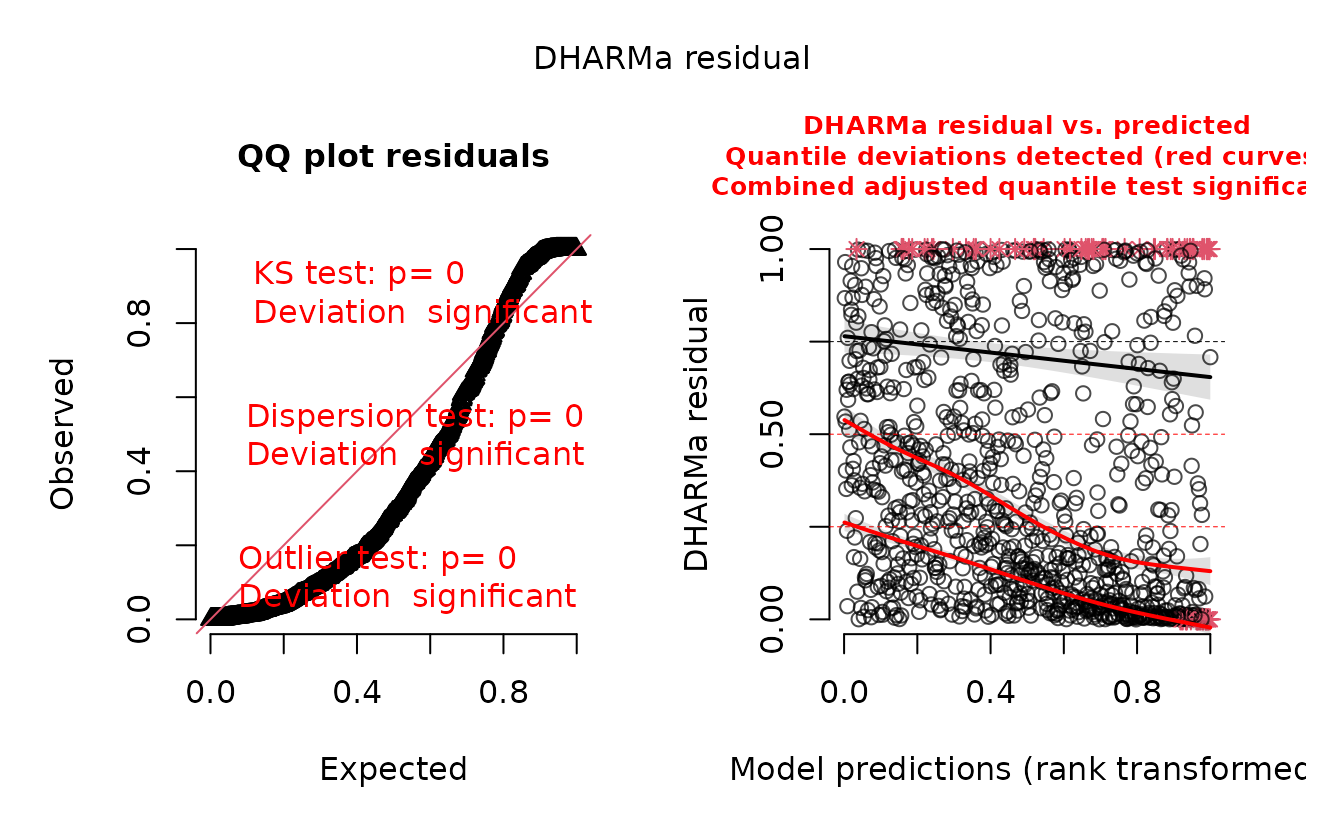

DHARMa::testResiduals(r_pois)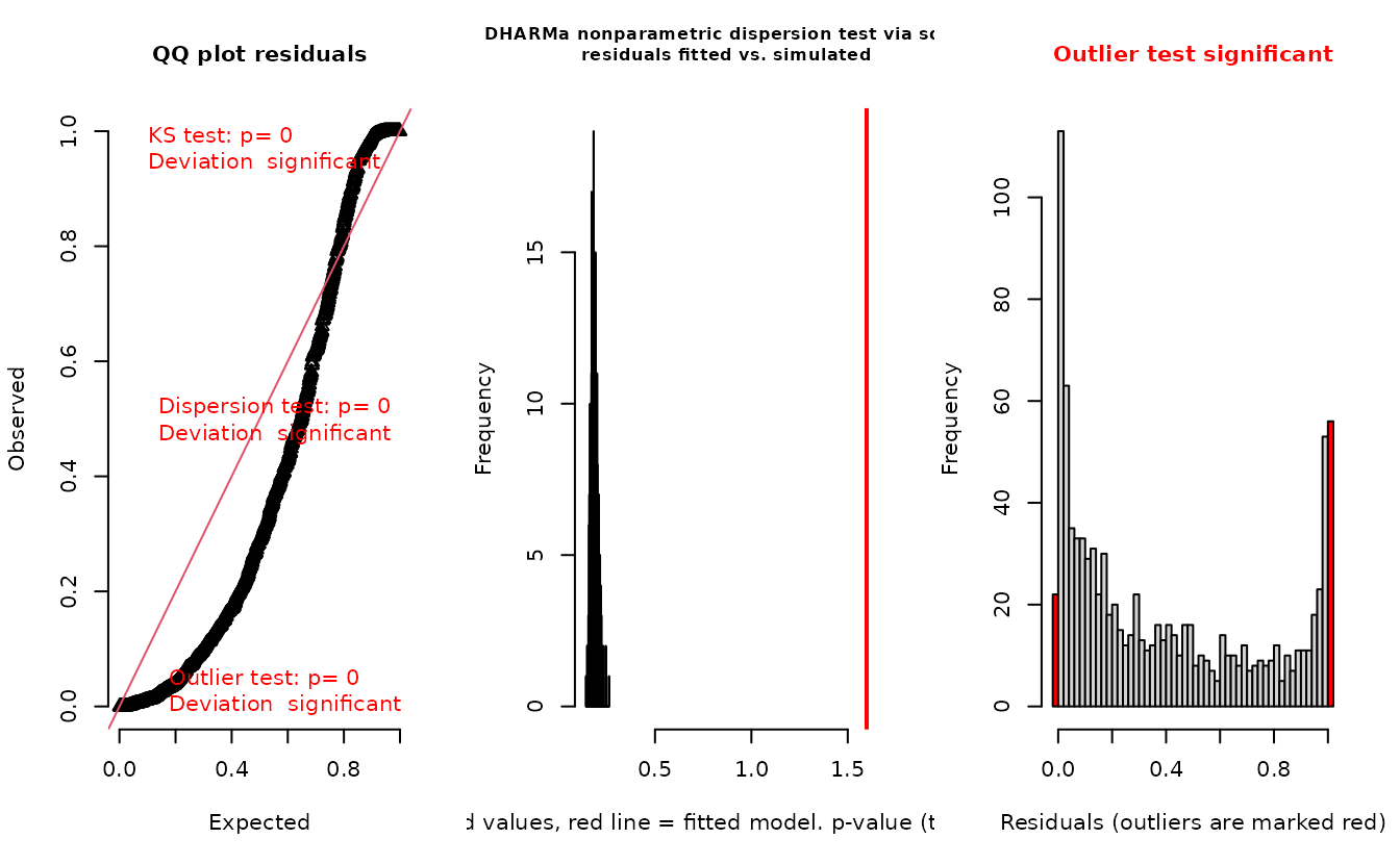

#> $uniformity
#> 
#>  Asymptotic one-sample Kolmogorov-Smirnov test
#> 
#> data:  simulationOutput$scaledResiduals
#> D = 0.23338, p-value < 2.2e-16
#> alternative hypothesis: two-sided
#> 
#> 
#> $dispersion
#> 
#>  DHARMa nonparametric dispersion test via sd of residuals fitted vs.
#>  simulated
#> 
#> data:  simulationOutput
#> dispersion = 8.6989, p-value < 2.2e-16
#> alternative hypothesis: two.sided
#> 
#> 
#> $outliers
#> 
#>  DHARMa outlier test based on exact binomial test with approximate
#>  expectations
#> 
#> data:  simulationOutput
#> outliers at both margin(s) = 111, observations = 1000, p-value <
#> 2.2e-16
#> alternative hypothesis: true probability of success is not equal to 0.003992016
#> 95 percent confidence interval:
#>  0.09219791 0.13212606
#> sample estimates:
#> frequency of outliers (expected: 0.00399201596806387 ) 
#>                                                  0.111
DHARMa::testSpatialAutocorrelation(r_pois, x = dat$X, y = dat$Y)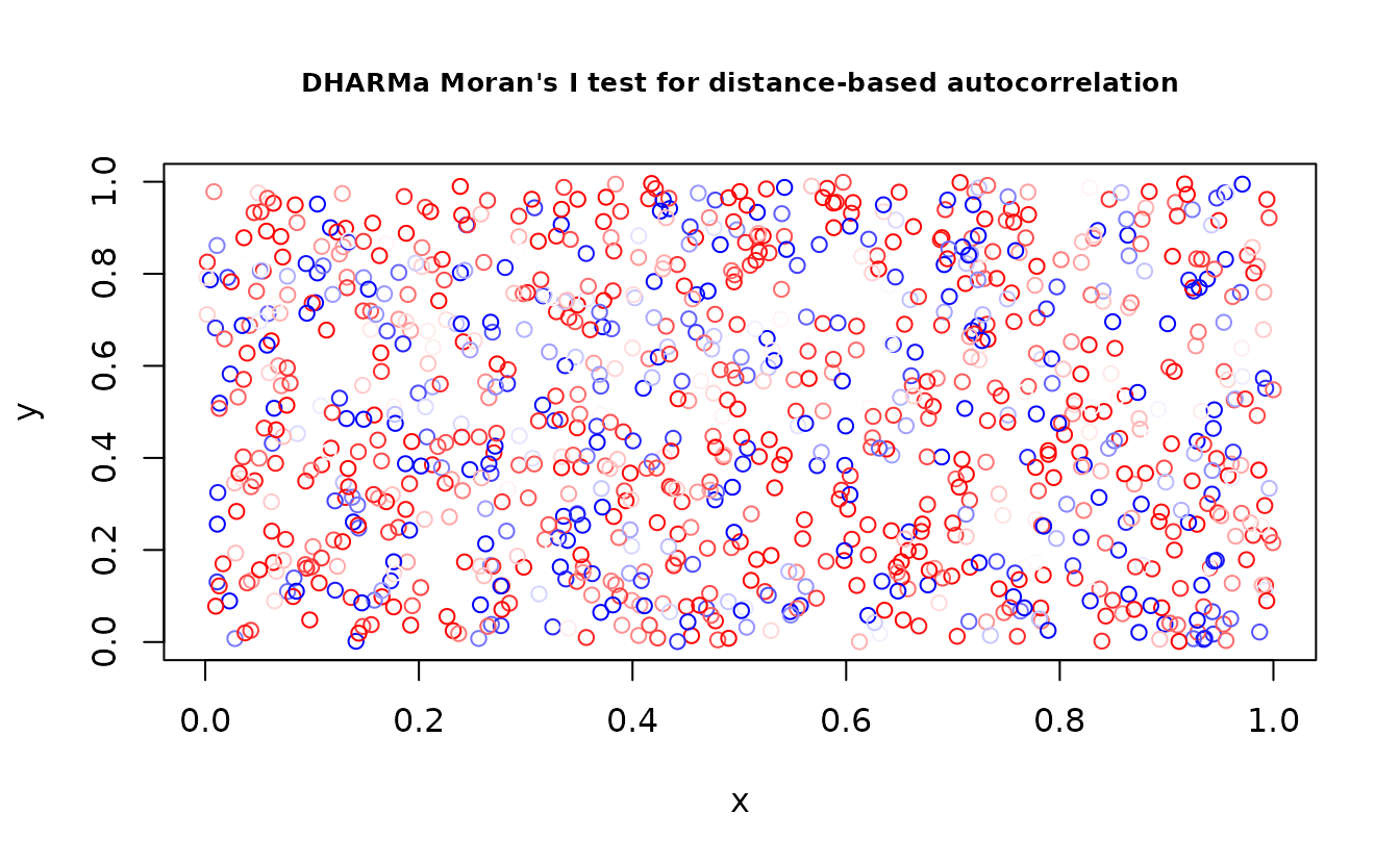

#> 
#>  DHARMa Moran's I test for distance-based autocorrelation
#> 
#> data:  r_pois
#> observed = -0.0022978, expected = -0.0010010, sd = 0.0026264, p-value =
#> 0.6215
#> alternative hypothesis: Distance-based autocorrelation
DHARMa::testZeroInflation(r_pois)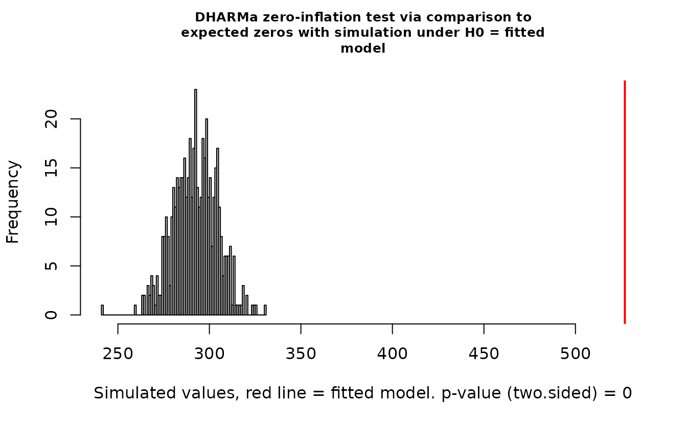

#> 
#>  DHARMa zero-inflation test via comparison to expected zeros with
#>  simulation under H0 = fitted model
#> 
#> data:  simulationOutput
#> ratioObsSim = 1.7999, p-value < 2.2e-16
#> alternative hypothesis: two.sided

In the QQ residual plots we clearly see evidence of overdispersion relative to the Poisson model. Note the values clumping near 1.0 on the observed axis and deviating downwards towards 0.0 observed. This is indicative of too many zeros and variance increasing too rapidly with the mean for the Poisson distribution, resulting in some large outlying values.

Let’s try the correct model:

r_nb2 <- dharma_residuals(s_nb2, fit_nb2, return_DHARMa = TRUE)
plot(r_nb2)

DHARMa::testZeroInflation(r_nb2)

#> 
#>  DHARMa zero-inflation test via comparison to expected zeros with
#>  simulation under H0 = fitted model
#> 
#> data:  simulationOutput
#> ratioObsSim = 1.0045, p-value = 0.908
#> alternative hypothesis: two.sided

Everything looks fine.

What about the model where we were missing a predictor?

r_nb2_miss <- dharma_residuals(s_nb2_miss, fit_nb2_miss, return_DHARMa = TRUE)
plot(r_nb2_miss)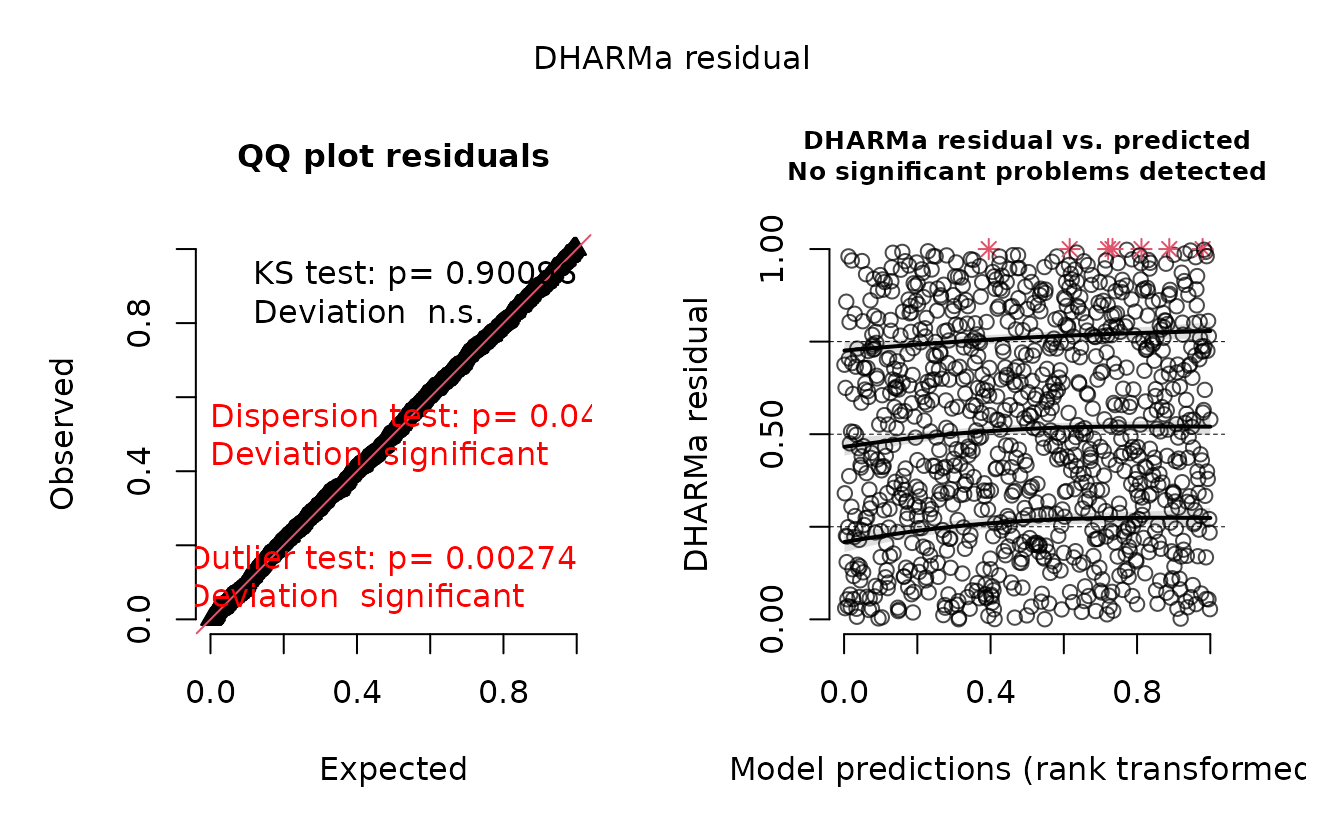

The plot on the right represents simulated residuals against the prediction without the random effects, which here is just an intercept. Let’s try plotting the residuals against the missing predictor:

DHARMa::plotResiduals(r_nb2_miss, form = dat$a1)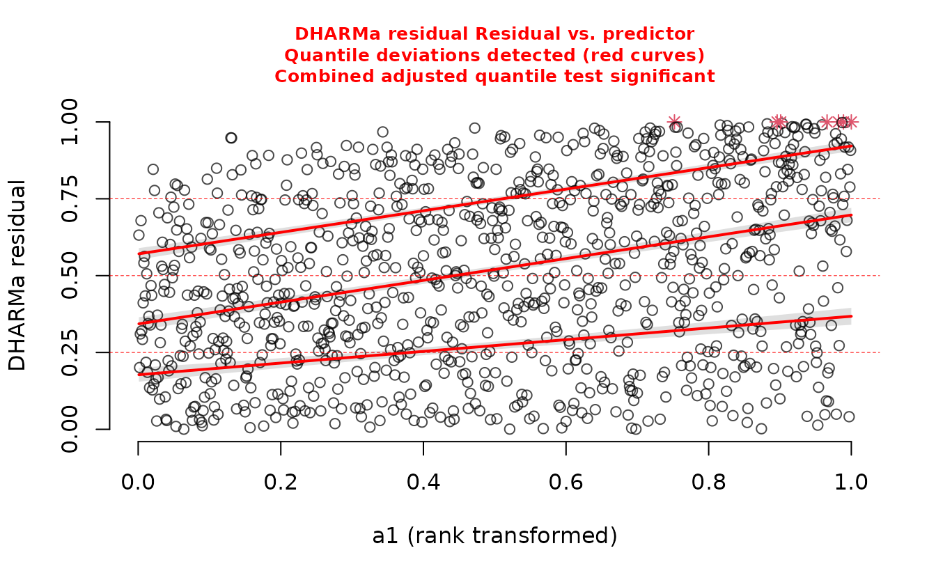

We can see a trend in the residuals against a1 because we omitted it from the model.

We can also see the difference in the log likelihood or the AIC:

AIC(fit_nb2_miss, fit_nb2)
#>              df      AIC
#> fit_nb2_miss  4 3642.665
#> fit_nb2       5 3480.904

AIC also supports including the a1 predictor.

For help interpreting the DHARMa residual plots, see vignette("DHARMa", package="DHARMa").

Extracting DHARMa residuals

We can extract the DHARMa residuals if we want to plot them ourselves. For example, let’s extract the DHARMa residuals from a model and make a QQ plot for each year:

pcod_dat <- pcod_2011
fit_pcod <- sdmTMB(
  density ~ factor(year), 
  time = "year",
  data = pcod_dat, 
  mesh = pcod_mesh_2011, 
  family = tweedie()
)
set.seed(1)

# make sure to set return_DHARMa = TRUE:
dh <- simulate(fit_pcod, nsim = 300, type = "mle-mvn") |> 
  dharma_residuals(fit_pcod, return_DHARMa = TRUE)

# add the DHARMa scaled residuals to the fitted data:
pcod_dat$scaled_residuals <- dh$scaledResiduals

# a small function to calculate the quantile-quantile values:
make_qq <- function(x) {
  u <- x$scaled_residuals
  n <- length(u)
  m <- seq_len(n) / (n + 1)
  z <- qqplot(m, u, plot.it = FALSE)
}

# apply our function to each year:
out <- group_by(pcod_dat, year) |> 
  group_split() |> 
  purrr::map_dfr(make_qq, .id = "year")

# plot it
ggplot(out, aes(x, y)) + 
  facet_wrap(vars(year)) + 
  geom_point() + 
  geom_abline(intercept = 0, slope = 1)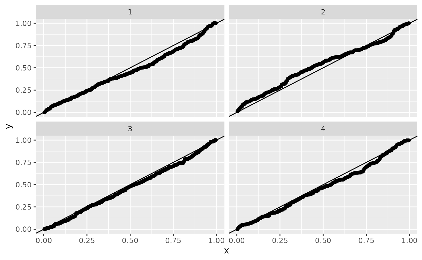

The need for one-sample residuals

The above used random effects drawn as if they were observed once.

The approach is described in Waagepetersen (2006) and is summarized nicely in an unexported function, oneSamplePosterior(), within TMB. Thygesen et al. (2017) also describe it in the context of one-sample MCMC residuals.

Here we will show why this is necessary.

We’ll start by simulating some data with Gaussian observation error and spatial and spatiotemporal random effects.

set.seed(123)
predictor_dat <- data.frame(
  X = runif(1000), Y = runif(1000),
  year = rep(1:5, each = 200)
)
mesh <- make_mesh(predictor_dat, xy_cols = c("X", "Y"), cutoff = 0.1)
sim_dat <- sdmTMB_simulate(
  formula = ~ 1,
  data = predictor_dat,
  time = "year",
  mesh = mesh,
  family = gaussian(),
  range = 0.3,
  sigma_E = 0.3,
  phi = 0.1,
  sigma_O = 0.4,
  seed = 1,
  B = 0.2 # intercept
)
fit <- sdmTMB(observed ~ 1, data = sim_dat, time = "year", mesh = mesh)

If we use the empirical Bayes (EB) random-effect values (the values of the random effects that maximize the log likelihood conditional on the estimated fixed effects), our residuals look off even though our model is perfectly matched to our simulated data:

set.seed(1)
r1 <- residuals(fit, type = "mle-eb")
qqnorm(r1);abline(0, 1)

ks.test(r1, pnorm)
#> 
#>  Asymptotic one-sample Kolmogorov-Smirnov test
#> 
#> data:  r1
#> D = 0.058629, p-value = 0.002067
#> alternative hypothesis: two-sided

Indeed, our test (incorrectly) rejects the null hypothesis that $r_1 \sim \operatorname{N}(0, 1)$, even though if the residuals are calculated correctly we know they do come from $\operatorname{N}(0, 1)$.

If instead we return to a single sample from the assumed MVN random-effect distribution, we get the “correct” residuals:

set.seed(1)
r2 <- residuals(fit, type = "mle-mvn")
qqnorm(r2);abline(0, 1)

ks.test(r2, pnorm)
#> 
#>  Asymptotic one-sample Kolmogorov-Smirnov test
#> 
#> data:  r2
#> D = 0.020639, p-value = 0.7879
#> alternative hypothesis: two-sided

Here, we would (correctly) fail to reject the hypothesis that $r_2 \sim \operatorname{N}(0, 1)$.

We could also sample that draw of random effects using MCMC (with the fixed effects still held at their MLEs), which relaxes our assumptions, but is much more time-intensive for large models.

samp <- sdmTMBextra::predict_mle_mcmc(fit, mcmc_iter = 400, mcmc_warmup = 200)
#> 
#> SAMPLING FOR MODEL 'tmb_generic' NOW (CHAIN 1).
#> Chain 1: 
#> Chain 1: Gradient evaluation took 0.002164 seconds
#> Chain 1: 1000 transitions using 10 leapfrog steps per transition would take 21.64 seconds.
#> Chain 1: Adjust your expectations accordingly!
#> Chain 1: 
#> Chain 1: 
#> Chain 1: Iteration:   1 / 400 [  0%]  (Warmup)
#> Chain 1: Iteration:  40 / 400 [ 10%]  (Warmup)
#> Chain 1: Iteration:  80 / 400 [ 20%]  (Warmup)
#> Chain 1: Iteration: 120 / 400 [ 30%]  (Warmup)
#> Chain 1: Iteration: 160 / 400 [ 40%]  (Warmup)
#> Chain 1: Iteration: 200 / 400 [ 50%]  (Warmup)
#> Chain 1: Iteration: 201 / 400 [ 50%]  (Sampling)
#> Chain 1: Iteration: 240 / 400 [ 60%]  (Sampling)
#> Chain 1: Iteration: 280 / 400 [ 70%]  (Sampling)
#> Chain 1: Iteration: 320 / 400 [ 80%]  (Sampling)
#> Chain 1: Iteration: 360 / 400 [ 90%]  (Sampling)
#> Chain 1: Iteration: 400 / 400 [100%]  (Sampling)
#> Chain 1: 
#> Chain 1:  Elapsed Time: 30.889 seconds (Warm-up)
#> Chain 1:                28.432 seconds (Sampling)
#> Chain 1:                59.321 seconds (Total)
#> Chain 1:
#> Warning: The largest R-hat is 1.09, indicating chains have not mixed.
#> Running the chains for more iterations may help. See
#> https://mc-stan.org/misc/warnings.html#r-hat
#> Warning: Bulk Effective Samples Size (ESS) is too low, indicating posterior means and medians may be unreliable.
#> Running the chains for more iterations may help. See
#> https://mc-stan.org/misc/warnings.html#bulk-ess
#> Warning: Tail Effective Samples Size (ESS) is too low, indicating posterior variances and tail quantiles may be unreliable.
#> Running the chains for more iterations may help. See
#> https://mc-stan.org/misc/warnings.html#tail-ess
r3 <- residuals(fit, type = "mle-mcmc", mcmc_samples = samp)
qqnorm(r3);abline(0, 1)

ks.test(r3, pnorm)
#> 
#>  Asymptotic one-sample Kolmogorov-Smirnov test
#> 
#> data:  r3
#> D = 0.024984, p-value = 0.5604
#> alternative hypothesis: two-sided

Here that gets us something similar, and we would (correctly) fail to reject the hypothesis that $r_3 \sim \operatorname{N}(0, 1)$.

A similar issue applies to simulation-based quantile residuals, as implemented in the DHARMa package.

set.seed(1)
simulate(fit, nsim = 500, type = "mle-eb") |>
  dharma_residuals(fit)
#> Warning: It is recommended to use `simulate.sdmTMB(fit, type = 'mle-mvn')` if simulating
#> for DHARMa residuals. See the description in ?residuals.sdmTMB under the types
#> of residuals section.

Instead we can use a draw from the random-effects “posterior” assuming an MVN distribution.

set.seed(1)
simulate(fit, nsim = 500, type = "mle-mvn") |>
  dharma_residuals(fit)

And now that looks correct.

However, what happens if we were to sample the random effects with each simulation?

set.seed(1)
s <- replicate(200, simulate(fit, nsim = 1, type = "mle-mvn"), simplify = "matrix")
attr(s, "type") <- "mle-mvn"
dharma_residuals(s, fit)

We get back to something with the wrong reference distribution for comparison. So, we need a single random effects sample per set of simulations.

How much this matters depends on the ratio of observation error variance vs. random effect variance

Let’s simulate data again, but with large observation error (phi here, which is the Gaussian error SD in this case) and smaller random-field variances (sigma_E and sigma_O):

set.seed(123)
sim_dat2 <- sdmTMB_simulate(
  formula = ~ 1,
  data = predictor_dat,
  time = "year",
  mesh = mesh,
  family = gaussian(),
  range = 0.3,
  sigma_E = 0.1, # smaller than before
  sigma_O = 0.1, # smaller than before
  phi = 0.5, # bigger than before
  seed = 1,
  B = 0.2 
)
fit2 <- sdmTMB(observed ~ 1, data = sim_dat2, time = "year", mesh = mesh)
sanity(fit2)
#> ✔ Non-linear minimizer suggests successful convergence
#> ✔ Hessian matrix is positive definite
#> ✔ No extreme or very small eigenvalues detected
#> ✔ No gradients with respect to fixed effects are >= 0.001
#> ✔ No fixed-effect standard errors are NA
#> ✔ No standard errors look unreasonably large
#> ✔ No sigma parameters are < 0.01
#> ✔ No sigma parameters are > 100
#> ✔ Range parameter doesn't look unreasonably large

set.seed(1)
r1 <- residuals(fit2, type = "mle-eb")
qqnorm(r1);abline(0, 1)

ks.test(r1, pnorm)
#> 
#>  Asymptotic one-sample Kolmogorov-Smirnov test
#> 
#> data:  r1
#> D = 0.021085, p-value = 0.7656
#> alternative hypothesis: two-sided

r2 <- residuals(fit2, type = "mle-mvn")
qqnorm(r2);abline(0, 1)

ks.test(r2, pnorm)
#> 
#>  Asymptotic one-sample Kolmogorov-Smirnov test
#> 
#> data:  r2
#> D = 0.016869, p-value = 0.9385
#> alternative hypothesis: two-sided

Now, it does not really matter because the “incorrect” random-effect distribution is swamped by the observation-error contribution to the distribution. Technically, the first set is “wrong” and the second set is “right”, but functionally we would come to a similar conclusion in this case.

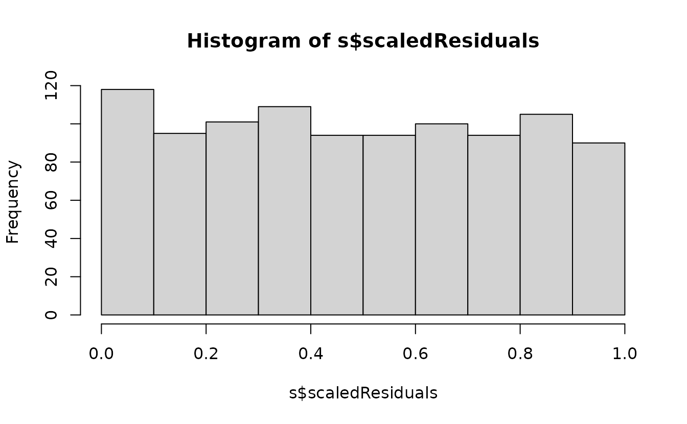
Notes on uniform vs. normal quantile residuals

The randomized quantile residuals in residuals.sdmTMB() are returned such that they will be normal(0, 1) if the model is consistent with the data. DHARMa residuals, however, are returned as uniform(0, 1) under those same circumstances. Both are valid, and which to use is largely a matter of preference, but it is important to appreciate how this changes the appearance of the expected residuals.

r2 <- residuals(fit2, type = "mle-mvn")

Analytical normal(0, 1):

hist(r2)

qqnorm(r2)
abline(0, 1)

ks.test(r2, pnorm)
#> 
#>  Asymptotic one-sample Kolmogorov-Smirnov test
#> 
#> data:  r2
#> D = 0.025614, p-value = 0.528
#> alternative hypothesis: two-sided

Analytical uniform(0, 1):

u <- pnorm(r2)
hist(u)

n <- length(u)
m <- seq_len(n) / (n + 1)
qqplot(m, u)
ks.test(u, punif)
#> 
#>  Asymptotic one-sample Kolmogorov-Smirnov test
#> 
#> data:  u
#> D = 0.025614, p-value = 0.528
#> alternative hypothesis: two-sided
abline(0, 1)

Simulation-based uniform(0, 1):

set.seed(1)
s <- simulate(fit2, nsim = 500, type = "mle-mvn") |>
  dharma_residuals(fit2, return_DHARMa = TRUE)
hist(s$scaledResiduals)

u <- s$scaledResiduals
m <- seq_len(length(u)) / (length(u)+ 1)
qqplot(m, u)
abline(0, 1)

ks.test(u, punif)
#> 
#>  Asymptotic one-sample Kolmogorov-Smirnov test
#> 
#> data:  u
#> D = 0.026, p-value = 0.5085
#> alternative hypothesis: two-sided

Simulation-based normal(0, 1):

set.seed(1)
s <- simulate(fit2, nsim = 1500, type = "mle-mvn") |>
  dharma_residuals(fit2, return_DHARMa = TRUE)
#> Simulating ■■■■■■■■■■■■■■■■■■■■■■■■■■■■■■■  100% | ETA:  0s
#> Simulating ■■■■■■■■■■■■■■■■■■■■■■■■■■■■■■■  100% | ETA:  0s
u <- s$scaledResiduals
r <- qnorm(u)
qqnorm(r)
abline(0, 1)

ks.test(u, punif)
#> 
#>  Asymptotic one-sample Kolmogorov-Smirnov test
#> 
#> data:  u
#> D = 0.028, p-value = 0.4131
#> alternative hypothesis: two-sided

Conclusions:

The normal(0, 1) residuals are probably more familiar to most people.

The normal(0, 1) residuals put more emphasis on the tails. This is both good and bad: it is easier to examine tail behaviour, but these residuals can often look “off” even when the model is fine (as in this example) because observations in the tails of the distribution are, by definition, rarely observed.

Uniform(0, 1) residuals give all data points equal visual weight and emphasize consistency of the overall distribution rather than the tails.

Either is valid, but you do need to adjust your expectations accordingly. For example, poor tail behaviour may look like a minor issue with uniform residuals; conversely, the tails of normal(0, 1) residuals are unlikely ever to look “perfect” without large sample sizes.

How do those randomized-quantile residuals work?

Let’s work through a simple example with the gamma distribution:

set.seed(1)
mu <- rep(2, 500)
phi <- 0.5
y <- rgamma(length(mu), shape = phi, scale = mu / phi)

To get quantile residuals, we transform those to uniform(0, 1) using pgamma() and then (optionally) convert those to normal(0, 1) with qnorm():

u <- pgamma(q = y, shape = phi, scale = mu / phi)
hist(u)

r <- qnorm(u)
hist(r)

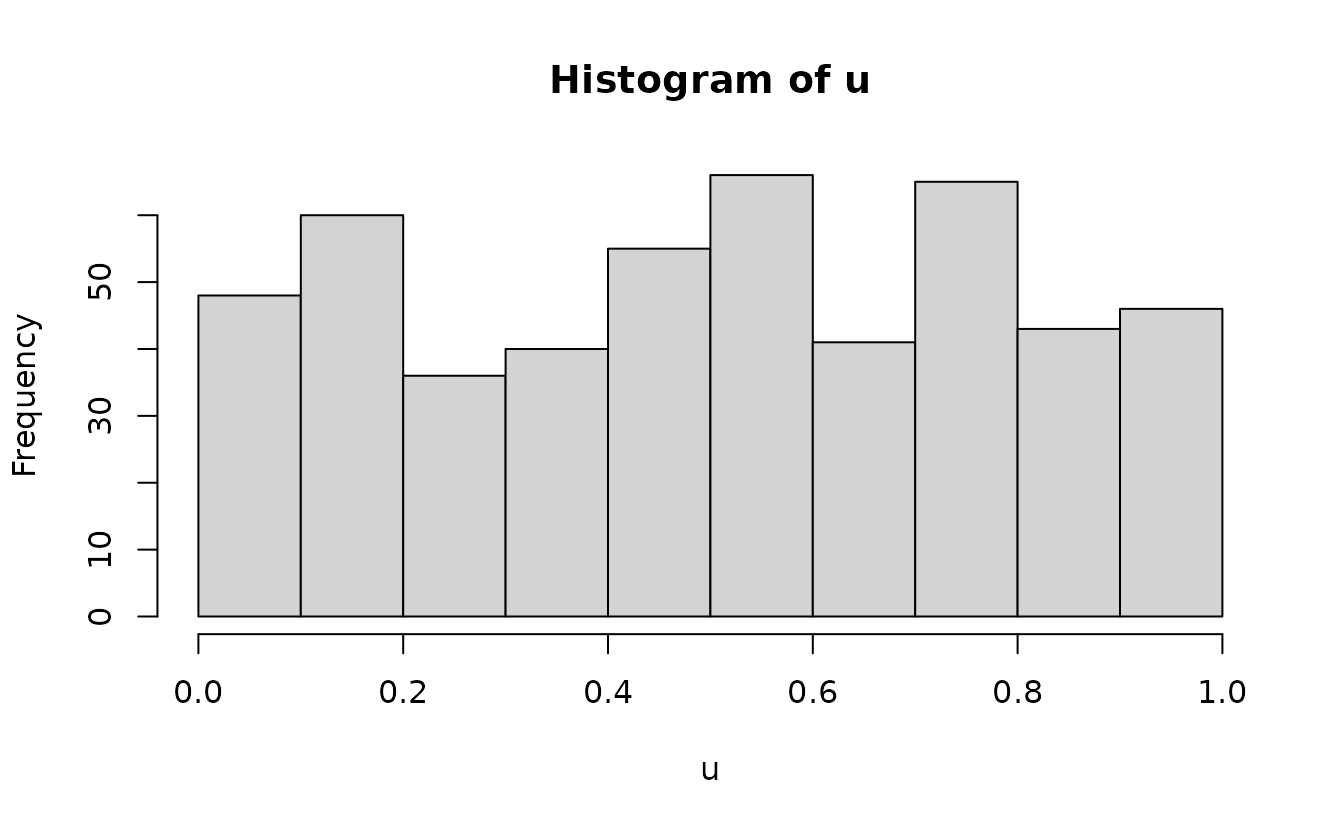
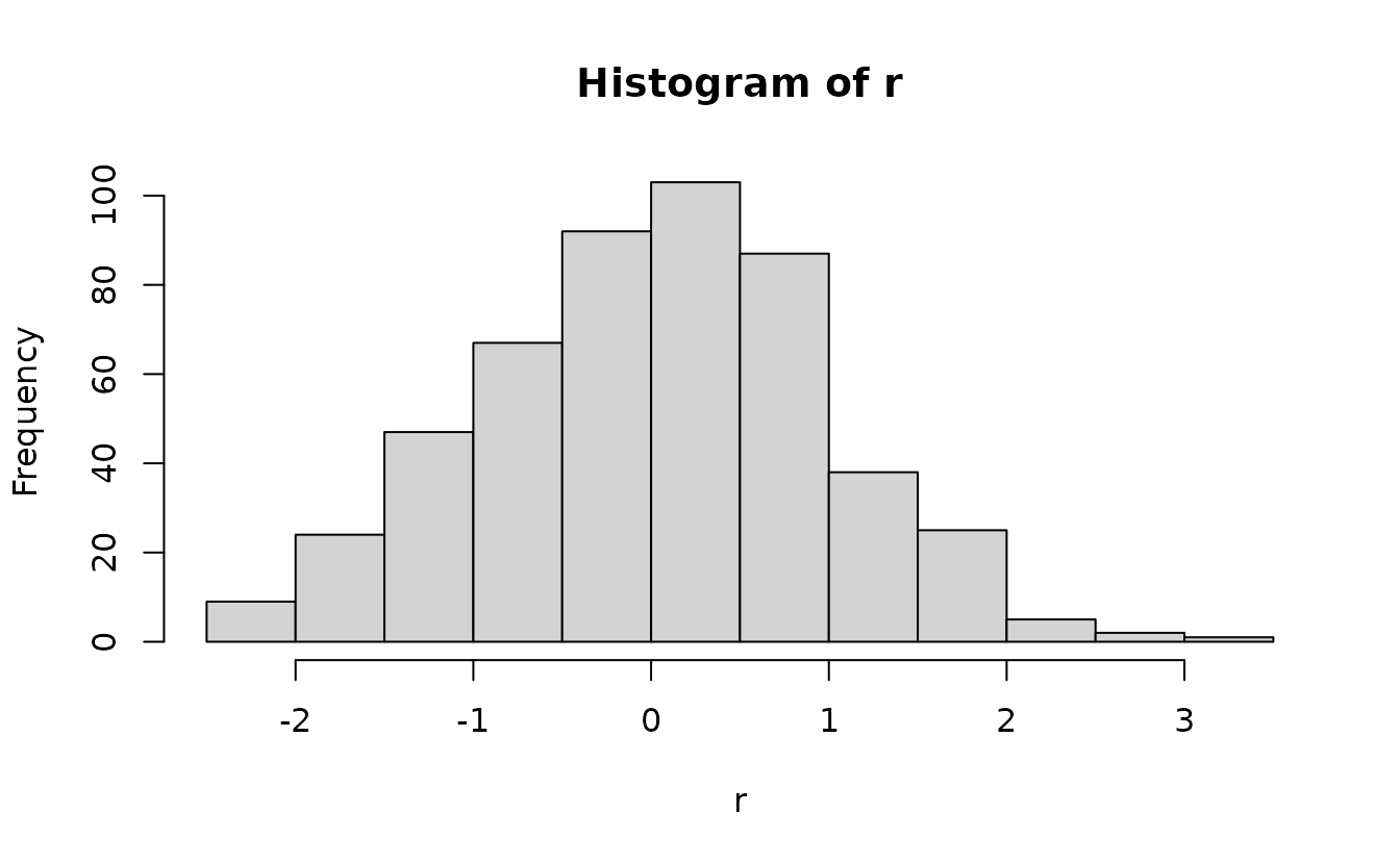
This works for any distribution as long as we can define the distribution function.

If we have integer values, we need to add randomization in an additional step. Let’s work with a Poisson sample:

set.seed(1)
mu <- rep(2, 500)
y <- rpois(length(mu), mu)

The gamma example above illustrated how we can use the distribution function (there pgamma()) to take a gamma-distributed variable and turn it into a uniformly distributed variable.

Now we need to do the same with the Poisson equivalent: ppois(). The ppois(y) function gives us the cumulative probability up to value y. Say we have a Poisson variable with a mean (lambda) of 5 and we have an observation with a value of 3. We can calculate the density up to the value of 3 as:

lambda <- 5
ppois(3, lambda)
#> [1] 0.2650259

That is the same as:

dpois(0, lambda) + dpois(1, lambda) + dpois(2, lambda) + dpois(3, lambda)
#> [1] 0.2650259

But if we naively apply ppois() to the observed values, we end up with discrete cumulative probabilities that are not very useful for comparing against a continuous uniform distribution.

hist(ppois(y, mu))

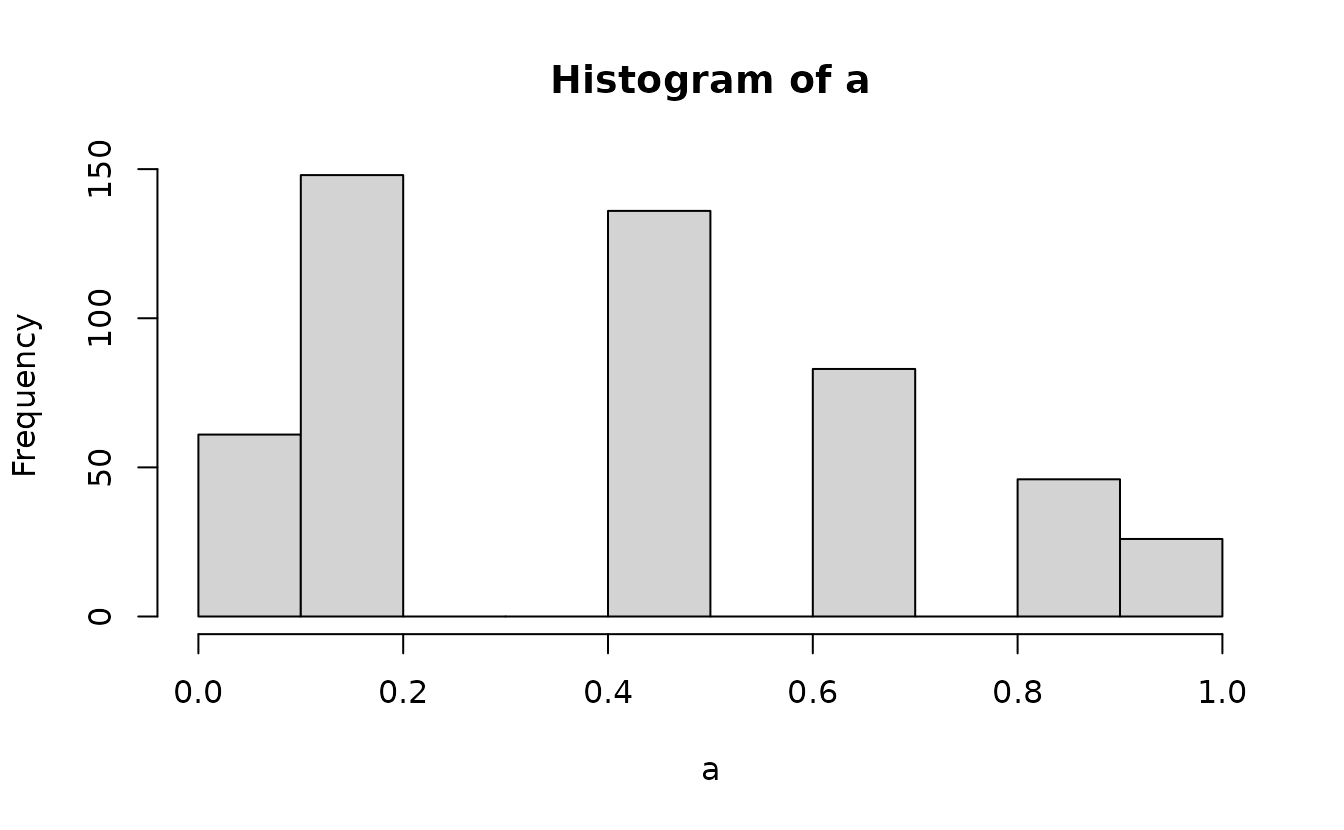
Instead, we need to get the cumulative probability up to the value below the one we observed and “fill in” the values up to the observed value with the desired uniformly distributed samples. First, get the cumulative probability up to the value below and up to the observed value:

a <- ppois(y - 1, mu)
hist(a)

b <- ppois(y, mu)
hist(b)

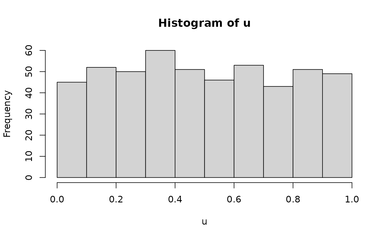
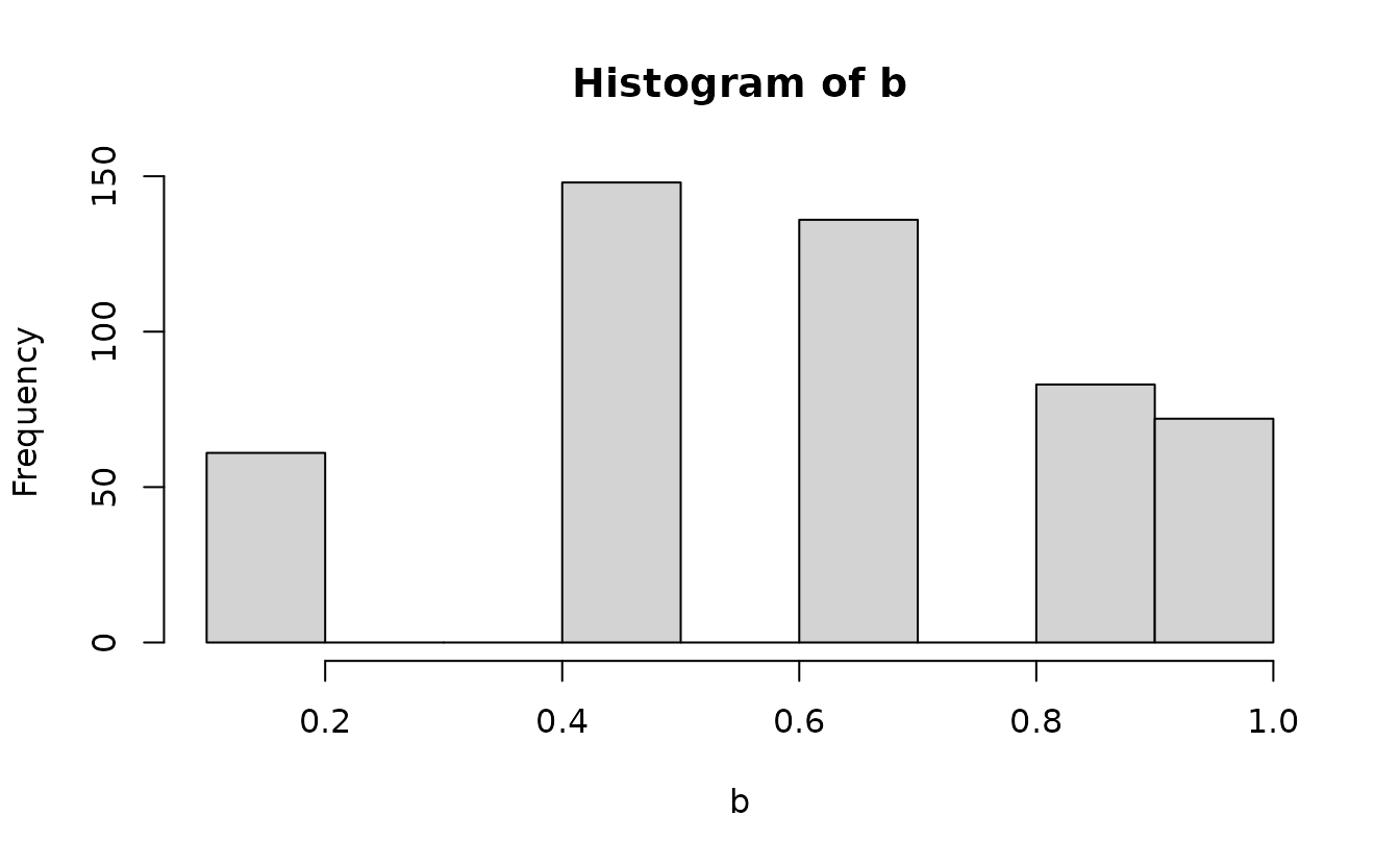
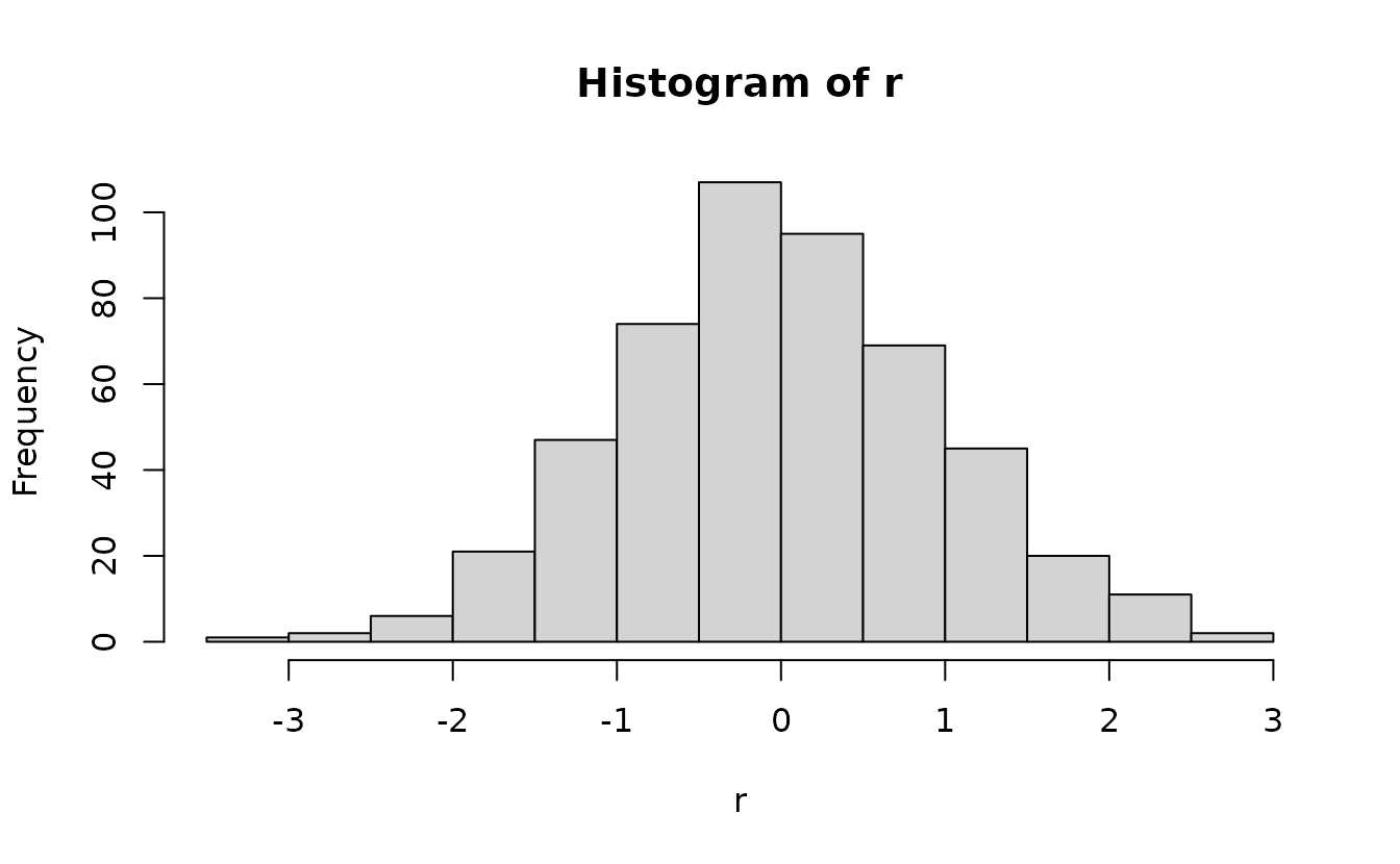
Then we can add randomization between these using runif() since our expectation is a uniform distribution at this stage to fill in the values between:

u <- runif(n = length(y), min = a, max = b)
hist(u)

Then we optionally apply qnorm():

r <- qnorm(u)
hist(r)

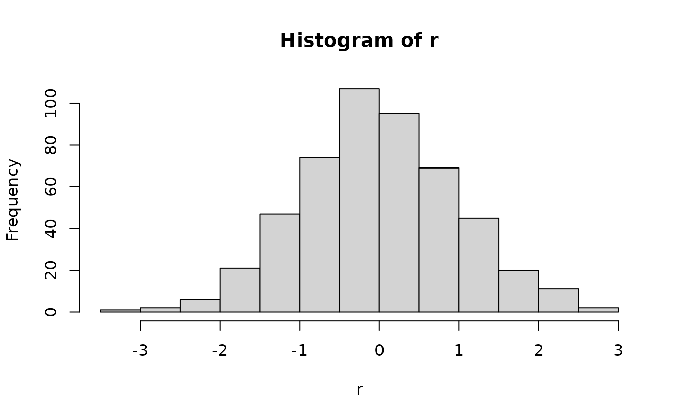
How do those simulation-based residuals work?

DHARMa uses simulation-based quantile residuals. As a result, we don’t need to define the quantile function analytically. So, instead of a line like this:

u <- pgamma(q = y, shape = phi, scale = mu / phi)

We simulate from our model repeatedly, see where our observation falls within the simulated values, and get our quantile that way. For example, instead of this:

pnorm(2.2, mean = 0.5, sd = 1)
#> [1] 0.9554345

we could do this:

set.seed(1)
s <- rnorm(1e6, 0.5, 1) # equivalent of simulate()ing from our model
mean(s < 2.2) # equivalent of pnorm()
#> [1] 0.955308

References

Dunn, P.K., and Smyth, G.K. 1996. Randomized Quantile Residuals. Journal of Computational and Graphical Statistics 5(3): 236–244.

Waagepetersen, R. 2006. A Simulation-Based Goodness-of-Fit Test for Random Effects in Generalized Linear Mixed Models. Scandinavian Journal of Statistics 33(4): 721–731.

Thygesen, U.H., Albertsen, C.M., Berg, C.W., Kristensen, K., and Nielsen, A. 2017. Validation of ecological state space models using the Laplace approximation. Environ Ecol Stat 24(2): 317–339.