Fitting multiple data types at once with sdmTMB • sdmTMB

Overview

This vignette shows how to fit a multi-family model where each row can use a different likelihood family. See Grüss & Thorson (2019) for the theory and citation for doing this in the context of fisheries survey data and for the context of including continuous positive data with Poisson-link families.

Multi-family models are experimental. The supported functions that work with multi-family models is deliberately small (fit, predict(), simulate()/DHARMa, tidy()/print(), and index-style derived quantities on a single-family grid); see Current limitations for the full list.

We will use the built-in dogfish dataset, but we’ll turn some rows into encounter/non-encounter and some into a count, just for the sake of an example. In reality, these are intended to come from different surveys or data sources.

We will:

Start with the dogfish dataset (catch weight),
Create three response types (binary, counts, and continuous),
Fit a multi-family model with binomial(cloglog), nbinom2(), and delta_lognormal(type = "poisson-link"),
Use log(area_swept) as an offset.

Important: only some families and links make sense to fit like this. Here, we make sure to use a cloglog link for the binomial and a Poisson-link for the delta-lognormal. The first linear predictor will represent an underlying (log) abundance. The binomial data observe that as a thinned count process via the cloglog. The NB2 data observe that as a count. The delta-lognormal data observe that as the ‘group’ count part of the Poisson-link formulation. The second linear predictor is then the ‘weight per group’ part of the Poisson-link formulation.

Data prep

Here we’ll create some fake count and encounter data from a dataset of catch weight for dogfish.

library(dplyr)
library(sdmTMB)
library(ggplot2)

set.seed(123)
data(dogfish, package = "sdmTMB")
dat <- dogfish |>
  mutate(
    log_depth = log(depth),
    data_type = sample(
      c("binomial", "nbinom2", "delta_lognormal"),
      size = n(),
      replace = TRUE
    )
  )

# Start from catch_weight and create:
# - binomial encounter indicator (0/1)
# - nbinom2 counts (scaled from catch_weight)
# - delta_lognormal response (raw catch_weight)
dat <- dat |>
  mutate(
    response = catch_weight,
    present_binom = as.integer(catch_weight > 0),
    response = ifelse(
      data_type == "binomial",
      present_binom,
      response
    ),
    response = ifelse(
      data_type == "nbinom2",
      pmax(0L, round(catch_weight / 10)),
      response
    )
  )

dat |>
  count(data_type)
#> # A tibble: 3 × 2
#>   data_type           n
#>   <chr>           <int>
#> 1 binomial          484
#> 2 delta_lognormal   499
#> 3 nbinom2           475

Model fit

We fit a multi-family model by passing a named list of families and a distribution_column that maps each row to a family name. Binomial would typically use a complementary log-log link for these types of integrated models. We also include a monitoring-program catchability effect using factor(data_type) in the first linear predictor, following the integrated monitoring programs approach described in Grüss and Thorson (2019).

Note that only delta_lognormal() has 2nd linear predictor, so we drop factor(data_type) in the 2nd set of main effects so the model is identifiable:

family_list <- list(
  binomial = binomial(link = "cloglog"),
  nbinom2 = nbinom2(),
  delta_lognormal = delta_lognormal(type = "poisson-link")
)

mesh <- make_mesh(dat, c("X", "Y"), cutoff = 10)

fit <- sdmTMB(
  formula = list(
    response ~ factor(data_type) + as.factor(year) + poly(log_depth, 2),
    response ~ factor(year) + poly(log_depth, 2) # omit factor(data_type) for the delta-positive component
  ),
  data = dat,
  family = family_list,
  distribution_column = "data_type",
  offset = log(dat$area_swept),
  spatial = "off",
  spatiotemporal = "off", # just for vignette building speed
  time = "year",
  mesh = mesh
)

fit
#> Model fit by ML ['sdmTMB']
#> Formula: list(response ~ factor(data_type) + as.factor(year) + poly(log_depth, 2), res...
#> Mesh: mesh (isotropic covariance)
#> Time column: year
#> Data: dat
#> Family: Multi-family (distribution column = 'data_type')
#> 
#> Linear predictor 1: -----------------------------------
#>  
#> Conditional model:
#>                                  coef.est coef.se
#> (Intercept)                          2.28    0.16
#> factor(data_type)delta_lognormal    -0.04    0.09
#> factor(data_type)nbinom2             1.29    0.12
#> as.factor(year)2006                  0.65    0.20
#> as.factor(year)2008                  0.45    0.20
#> as.factor(year)2010                  0.75    0.19
#> as.factor(year)2012                 -0.19    0.19
#> as.factor(year)2014                 -0.15    0.20
#> as.factor(year)2016                  0.16    0.20
#> as.factor(year)2018                  0.15    0.18
#> as.factor(year)2021                 -0.88    0.21
#> as.factor(year)2022                 -0.26    0.20
#> poly(log_depth, 2)1                  2.19    1.91
#> poly(log_depth, 2)2                -31.90    2.25
#> 
#> 
#> Linear predictor 2: -----------------------------------
#>  
#> Conditional model:
#>                     coef.est coef.se
#> (Intercept)             4.88    0.39
#> factor(year)2006       -0.74    0.46
#> factor(year)2008       -2.01    0.46
#> factor(year)2010       -1.03    0.46
#> factor(year)2012       -0.89    0.48
#> factor(year)2014       -1.36    0.46
#> factor(year)2016       -1.85    0.48
#> factor(year)2018       -1.79    0.45
#> factor(year)2021       -1.82    0.48
#> factor(year)2022       -2.25    0.49
#> poly(log_depth, 2)1    -2.16    4.20
#> poly(log_depth, 2)2   -16.02    4.44
#> 
#> Families:
#>  Linear predictor 1 Linear predictor 2 Dispersion param
#>   binomial(cloglog)                                    
#>        nbinom2(log)                                0.27
#>       binomial(log)     lognormal(log)             1.53
#> 
#> ML criterion at convergence: 3304.629
#> 
#> See ?tidy.sdmTMB to extract these values as a data frame.

Prediction grid and index

We can make predictions on the wcvi_grid and calculate an annual index with get_index(). For a multi-family model, newdata must include the distribution_column to indicate which family to use for each row. We should use a single family for the index so that we are calculating the index for one data type/survey. Here we calculate the index for the delta-lognormal component. I.e., we are calculating a biomass index.

years <- sort(unique(dat$year))

nd <- replicate_df(wcvi_grid, "year", years) |>
  mutate(
    log_depth = log(depth),
    data_type = "delta_lognormal",
    area_swept = 1, # 1 km^2, i.e. offset = log(1) = 0
    cell_area = 4 # 2 km x 2 km here
  )

index <- get_index(
  fit,
  newdata = nd,
  offset = log(nd$area_swept),
  area = "cell_area"
)
head(index)
#>   year      est      lwr      upr  log_est        se se_natural  type
#> 1 2004 19662959  9117796 42404100 16.79425 0.3921034    7709912 index
#> 2 2006 18080450 10863955 30090578 16.71034 0.2598930    4698982 index
#> 3 2008  4118518  2420208  7008567 15.23100 0.2712499    1117147 index
#> 4 2010 14768665  8761005 24895943 16.50802 0.2664320    3934845 index
#> 5 2012  6699294  3748556 11972752 15.71751 0.2962459    1984638 index
#> 6 2014  4347924  2554680  7399926 15.28521 0.2713170    1179666 index

ggplot(index, aes(year, est)) +
  geom_pointrange(aes(ymin = lwr, ymax = upr))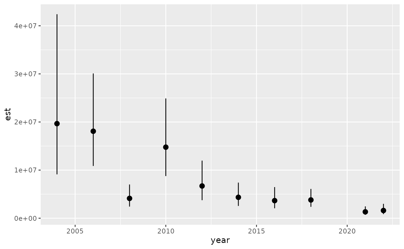

Prediction standard errors

Multi-family models support standard errors via se_fit = TRUE when making predictions. Standard errors are computed for each row using TMB’s delta method in link space.

You can get standard errors when the prediction grid contains multiple families. Each row’s SE corresponds to that row’s specific prediction and family:

# Prediction grid with mixed families
nd <- data.frame(log_depth = seq(
  log(min(dogfish$depth)),
  log(max(dogfish$depth)),
length.out = 100
))
nd$year <- dogfish$year[1] # pick a year here

nd_mixed <- replicate_df(
  nd, "data_type",
  c("binomial", "nbinom2", "delta_lognormal")
)

pred_mixed <- predict(
  fit,
  newdata = nd_mixed,
  re_form = NA,
  se_fit = TRUE,
  type = "link"
)

head(pred_mixed)
#>   log_depth year data_type        est       est1 est2    est_se
#> 1  3.761200 2004  binomial -1.1518911 -1.1518911   NA 0.3135759
#> 2  3.790767 2004  binomial -0.9686105 -0.9686105   NA 0.3028221
#> 3  3.820335 2004  binomial -0.7895247 -0.7895247   NA 0.2924645
#> 4  3.849902 2004  binomial -0.6146336 -0.6146336   NA 0.2825078
#> 5  3.879469 2004  binomial -0.4439373 -0.4439373   NA 0.2729568
#> 6  3.909036 2004  binomial -0.2774358 -0.2774358   NA 0.2638160

SEs are computed for each row according to its family

ggplot(pred_mixed, aes(log_depth, est)) +
  geom_ribbon(aes(ymin = est - 2 * est_se, ymax = est + 2 * est_se), fill = "grey80") +
  geom_line() +
  facet_wrap(~data_type)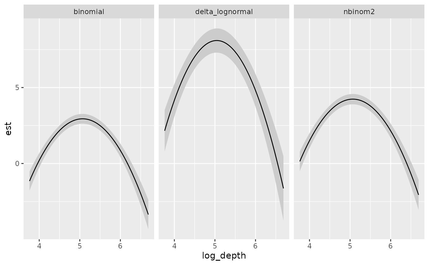

Important notes on standard errors

Link space: Standard errors are always in link space. type = "response" with se_fit = TRUE returns an error, as for any sdmTMB model.
Different link spaces per row: When your prediction grid contains multiple families, the est_se column contains SEs in potentially different link spaces (e.g., logit for binomial rows, log for count families). This is fine because the SEs are row-specific and correspond to each row’s prediction.
Delta families: For delta family rows, the combined prediction est has a standard error that accounts for uncertainty in both the encounter and positive components, computed using TMB’s delta method. This SE is generally different from either component’s SE alone (est1_se or est2_se). The est is presented in log space.

Current limitations

Multi-family models are intended to support the main fit, prediction, simulation, and index workflows. Some downstream helpers are still intentionally unsupported.

For residual diagnostics, the supported approach is simulation-based residuals with [simulate.sdmTMB()] and [dharma_residuals()]. This works for multi-family models and is the recommended workaround for the unsupported residuals.sdmTMB() method.

Function or feature	Multi-family status	Workaround or note
`residuals()`	Not supported	Use `simulate(fit, nsim = ..., type = "mle-mvn") \|> dharma_residuals(fit)` for simulation-based residual diagnostics.
`sigma()`	Not supported	Inspect family-specific parameters with `tidy()` or model summaries instead.
`deviance()`	Not supported	Use likelihood-based comparisons, simulation-based checks, or out-of-sample predictive checks instead.
`project()`	Not supported	Predict on the target grid directly with `predict()` and include `distribution_column` in `newdata`.
`emmeans()`	Not supported	Use `predict()` on custom `newdata` grids and summarize contrasts manually.
`plot_smooth()`	Not supported	Use direct `predict()` calls on custom grids or other custom plotting workflows.
`visreg::visreg()`, `visreg_delta()`	Not supported	Use direct `predict()` calls on custom grids.
`spread_sims()` / `gather_sims()`	Not supported	Use `predict(..., nsim = ...)` or `simulate()` draws directly.
`sdmTMB_cv()`	Not supported	Roll cross validation by hand.
`cAIC()`	Not supported	Use `AIC()` (marginal) or likelihood-based comparisons instead.
`do_index = TRUE` inside `sdmTMB()`	Not supported	Fit first, then call `get_index(fit, newdata = ...)` with the prediction grid and `distribution_column`.
`dispformula`	Not supported	Use `dispformula = ~ 1`. If your main goal is to allow different family-level auxiliary parameters across data sources (for example separate `phi` values), one workaround is to define separate named entries in `family = list(...)` even when they use the same likelihood family/link, and route rows with `distribution_column`.
`covariate_diffusion`	Not supported	No direct workaround within multi-family models yet.
Families outside the supported multi-family set	Not supported	Multi-family mode currently supports `gaussian()`, `binomial()`, `poisson()`, `nbinom1()`/`nbinom2()`, `tweedie()`, `betabinomial()`, and delta families built on Gamma, lognormal, or gengamma (standard or Poisson-link). Other families (e.g. `_mix()`, `ordbeta()`, `student()`) can still be fit as ordinary single-family models.

References

Grüss, A. & Thorson, J.T. (2019). Developing spatio-temporal models using multiple data types for evaluating population trends and habitat usage. ICES Journal of Marine Science, 76, 1748–1761.